

Direct elicitation in 1D#
import matplotlib.pyplot as plt
import numpy as np

import preliz as pz
pz.style.use("preliz-doc")
From intervals to maximum entropy distributions#
For some priors in a model, we may know or assume that most of the mass is within a certain interval. This information is useful for determining a suitable prior, but this information alone may not be enough to obtain a unique set of parameters. The following figure shows Beta distributions with 90% of the mass between 0.1 and 0.7, the dot represent the mode of the distribution. As you can see even when all these distributions satisfies that restraint they convey very different prior knowledge.
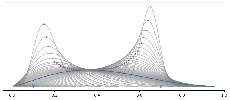
We can add one more condition, one that is very general. We can maximize the entropy. Given two distributions the one with more entropy is the less informative one. Loosely speaking, is the most “spread” one. In the previous figure, the blue line is the one with more entropy. Having priors with maximum entropy makes sense as this guarantees that we have the less informative distribution, given a set of constraints.
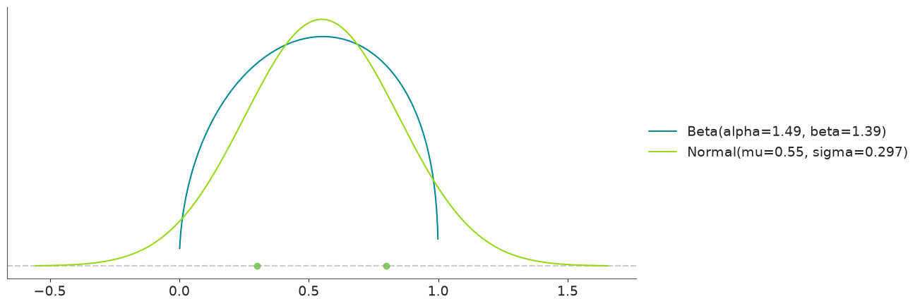
In PreliZ we can compute maximum entropy priors using the function maxent. The first argument is a PreliZ
distribution.
pz.maxent(pz.Beta(), lower=0.3, upper=0.8, mass=0.6)
pz.maxent(pz.Normal(), lower=0.3, upper=0.8, mass=0.6);
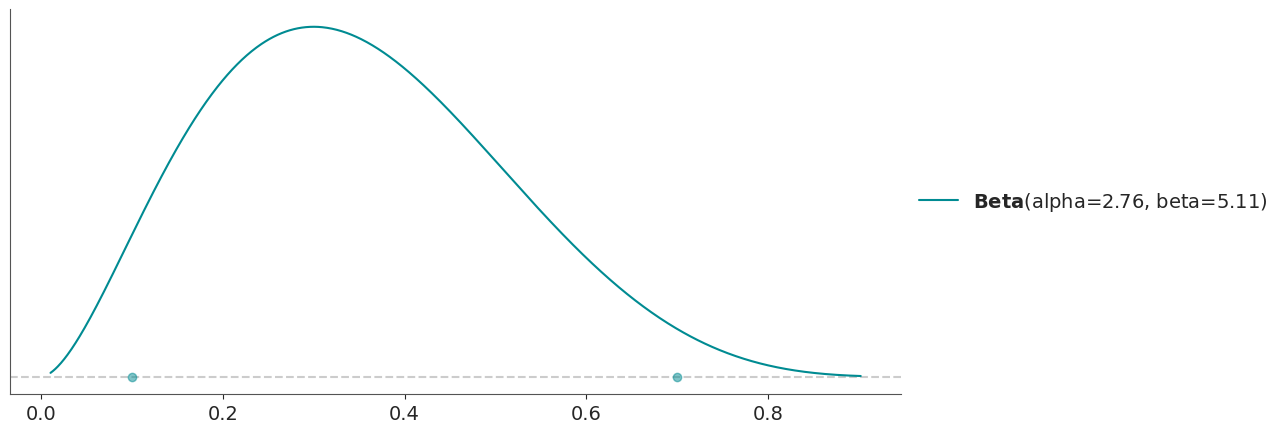
Usually, we pass uninitialized distribution to maxent. But we can also pass partially initialized distribution. This
is useful when we want to keep one or more parameters fixed. For instance, we may want to find a Gamma distribution with
a mean of 4 and with 90% of the mass between 1 and 10.
pz.maxent(pz.Gamma(mu=4), 1, 10, 0.9);
If you pass a distribution with all the parameters specified, like pz.Gamma(mu=4, sigma=1), you will get an error
saying “All parameters are fixed, at least one should be free”.
Many functions in PreliZ update distribution in place, maxent is no exception. So sometimes it is best to first
instantiate a distribution, and they use it, like this:
dist = pz.Gamma(mu=4)
pz.maxent(dist, 1, 10, 0.9);

this will allow us to keep working with dist, for instance to get its parameters
dist.alpha, dist.beta
(np.float64(2.341680163267631), np.float64(0.5854200408169078))
Sometimes we may want to fix some property of a distribution, that we can not fix directly by fixing a parameter. For
instance, we may want to fix the mode. We can do this by passing a proper tuple to fixed_stat.
dist = pz.Beta()
pz.maxent(dist, 0.1, 0.7, 0.94, fixed_stat=("mode", 0.3))
dist.mode()
array(0.29999997)
Other values that can be passed to fixed_stat are “mean”, “mode”, “median”, “variance”, “std”, “skewness” or “
kurtosis”.
Unsatisfiable constraints and over-restrictive constraints#
It’s important to recognize that there might not be a distribution that satisfies all our constraints. If the difference between the requested and computed masses within the interval exceeds a threshold, PreliZ will issue a warning. This helps us determine whether the computed distribution is still useful or if the inputs need to be adjusted.
On the other hand, we can also have over-restrictive constraints. For instance, if we ask for a Beta distribution with 90% of the mass between 0.1 and 0.7 and a mode of 0.5. We have enough information to determine the distribution, even without maximizing the entropy. In this case, PreliZ will just return the distribution that satisfies all the constraints without complaining.
dist = pz.Normal()
pz.maxent(dist, -2, 2, 0.9, fixed_stat=("median", 2), plot=False)
Normal(mu=1.94, sigma=0.0344)
| Kind | continuous |
| Support | (-inf, inf) |
| Mean | 1.9 |
| Std | 0.034 |
| Parametrizations | (mu, sigma), (mu, tau) |
PyMC interoperability#
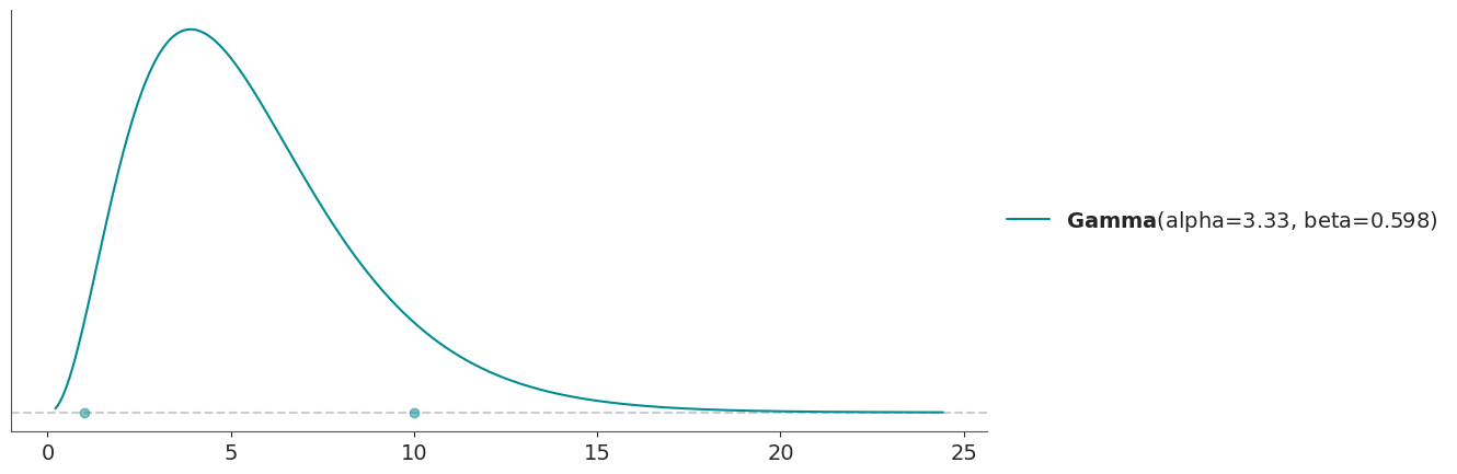
We can also use PyMC distributions with maxent, assuming we have PyMC installed. One difference is that we need to explicitly pass np.nan for the parameters we want to estimate. So we can not pass uninitialized distributions as we do with PreliZ distributions.
import pymc as pm

dist = pm.Gamma.dist(np.nan, np.nan)
new_dist, _ = pz.maxent(dist, 1, 10, 0.9);
new_dist
Gamma(alpha=3.33, beta=0.598)
| Kind | continuous |
| Support | (0, inf) |
| Mean | 5.6 |
| Std | 3.1 |
| Parametrizations | (alpha, beta), (mu, sigma) |
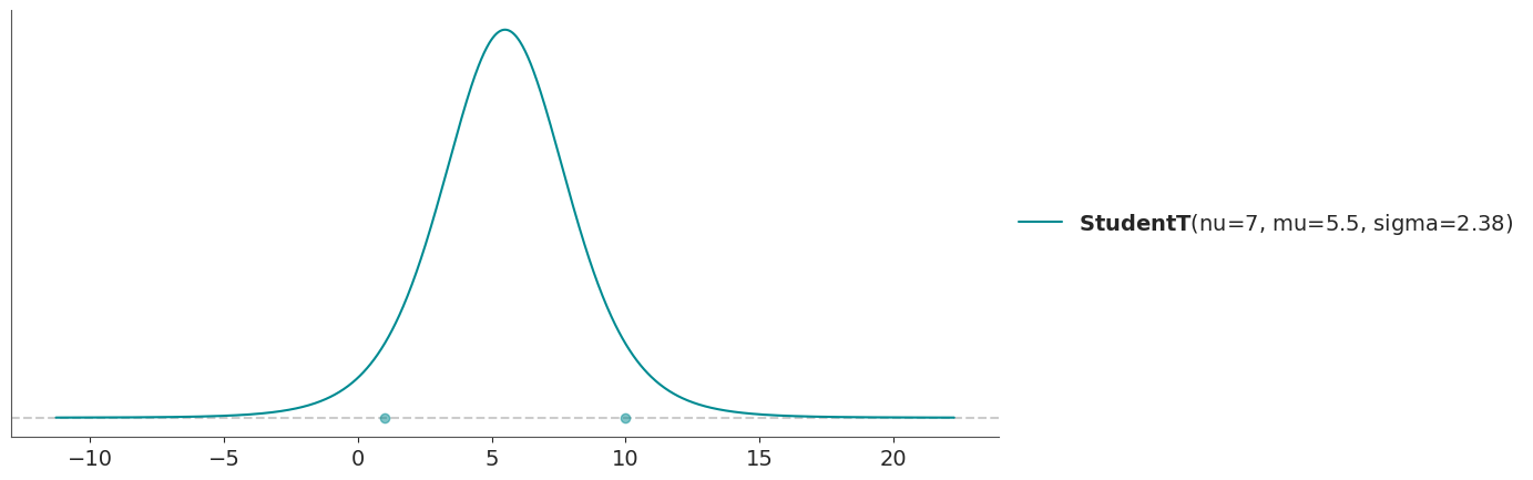
And if we want to fix some parameters we just pass their values instead of np.nan.
dist = pm.StudentT.dist(nu=7, mu=np.nan, sigma=np.nan)
pz.maxent(dist, 1, 10, 0.9);
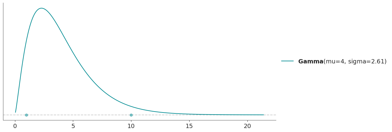
The caveat, is that fixing the parameters for PyMC distributions only works properly for the “canonical” parameters. For example, for the Gamma it will work as expected for alpha or beta but not for mu or sigma. So with PyMC distributions it is better to use fixed_params to fix parameters by name.
dist = pm.Gamma.dist(np.nan, np.nan)
new_dist, _ = pz.maxent(dist, 1, 10, 0.9, fixed_params={"mu": 4});
new_dist
Gamma(mu=4, sigma=2.61)
| Kind | continuous |
| Support | (0, inf) |
| Mean | 4 |
| Std | 2.6 |
| Parametrizations | (alpha, beta), (mu, sigma) |

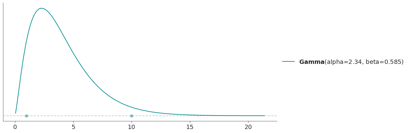
In this case we can also use fixed_stat to fix the mean, as both ways are equivalent for the Gamma distribution.
dist = pm.Gamma.dist(np.nan, np.nan)
new_dist, _ = pz.maxent(dist, 1, 10, 0.9, fixed_stat=("mean", 4));
new_dist
Gamma(alpha=2.34, beta=0.585)
| Kind | continuous |
| Support | (0, inf) |
| Mean | 4 |
| Std | 2.6 |
| Parametrizations | (alpha, beta), (mu, sigma) |
PyMC-extras interoperability#
We can pass Prior objects from PyMC-extras to maxent (and other functions), assuming we have PyMC-extras installed. As long as the resulting distribution is implemented in PreliZ, it will as expected,for instance we can partially initialize a Prior as a regular PreliZ distribution:
from pymc_extras.prior import Prior

dist = Prior("Gamma", mu=4)
pz.maxent(dist, 1, 10, 0.9);

From quartiles to distributions#
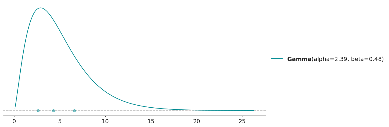
One alternative to maxent is to define a distribution by its quartiles, that
is by the 3 points which divides the distribution into 4 parts each with 25% of the total mass.
pz.quartile(pz.Gamma(), 2.6, 4.3, 6.6);
In many aspects quartile works similarly to maxent, we can also fix parameters, either by partially initializing PreliZ distributions or by using fixed_params. For PyMC distributions it’s better to use fixed_params.
From quartiles to distributions interactively#
Another function that allows to specify distribution in terms of quartiles is quartile_int. This is like quartile,
but it is interactive and we can pass a list of distribution families. The function will return the closest 1D
distribution to that input.
%matplotlib widget
pz.QuartileInt(1, 2, 3, ["StudentT", "TruncatedNormal", "BetaScaled"]);
As you can see, to run this function we first need to call the matplotlib widget magic, we also needs to have
ipywidgets installed (an optional requirement of PreliZ).
Notice that to specify the list of available distributions, we pass a list of strings, instead of a list of PreliZ’s
distributions. The params box, allows us to fix parameters for one or more distributions.
If you are unable to run the previous cell, you can get a glimpse of quartile_int from this gif
Before continuing we close the interactive figure and reinitialize the standard backend.
plt.close()
%matplotlib inline
From samples to maximum likelihood distributions#
For some problems, we may have data that we can use to inform priors. One way to do it is to fit the data to some parametric family of distributions. We can then use a maximum likelihood estimate to get the distribution with the best fit. To rank the distributions we use the Akaike Criterion, which includes a penalization term related to the number of parameters of each distribution.
# In a real scenario this will be some data and not a sample from a PreliZ distribution
sample = pz.StudentT(4, 0, 1).rvs(1000)

dist0 = pz.StudentT()
dist1 = pz.Normal()
dist2 = pz.Laplace()
pz.mle([dist0, dist1, dist2], sample, plot=3);  # we ask to plot all 3 distributions
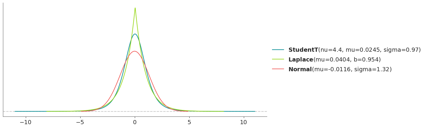
By default pz.mle only plots the best match, but here we decided to get a plot with the 3 fitted distributions. As
with maxent the distributions are updated in place so we can get access to them.
dist0
StudentT(nu=3.57, mu=0.0496, sigma=0.994)
| Kind | continuous |
| Support | (-inf, inf) |
| Mean | 0.05 |
| Std | 1.5 |
| Parametrizations | (nu, mu, sigma), (nu, mu, lam) |
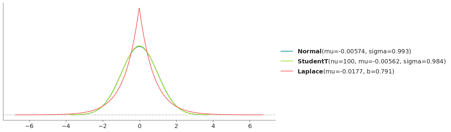
# In a real scenario this will be some data and not a sample from a PreliZ distribution
sample = pz.StudentT(5000, 0, 1).rvs(1000)

dist0 = pz.StudentT()
dist1 = pz.Normal()
dist2 = pz.Laplace()
pz.mle([dist0, dist1, dist2], sample, plot=3);  # we ask to plot all 3 distribution
From one distribution to another#
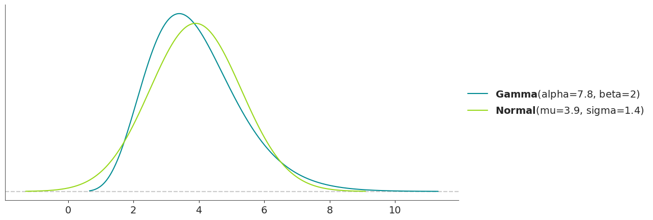
Moment matching is a technique that allows us to approximate a distribution with another one by matching a set of moments (like mean and variance). For instance, we may want to approximate a known Gamma distribution with a Normal distribution by matching the first two moments.
pz.match_moments(pz.Gamma(7.8, 2),
                   pz.Normal(),
                   )
(Normal(mu=3.9, sigma=1.4), <Axes: >)
By default, match_moments matches the first two moments (mean and variance). But we can also match other moments, like
skewness and kurtosis, by passing the moments argument.
We can also match distributions by their quantiles instead of their moments. This may be useful when the moments are not defined, or simply when we need to match specific quantiles. For instance, we can approximate a known Weibull distribution with a LogNormal distribution.
pz.match_quantiles(pz.Weibull(3.5, 2),
                   pz.LogNormal(),
                   )
(LogNormal(mu=0.571, sigma=0.327), <Axes: >)
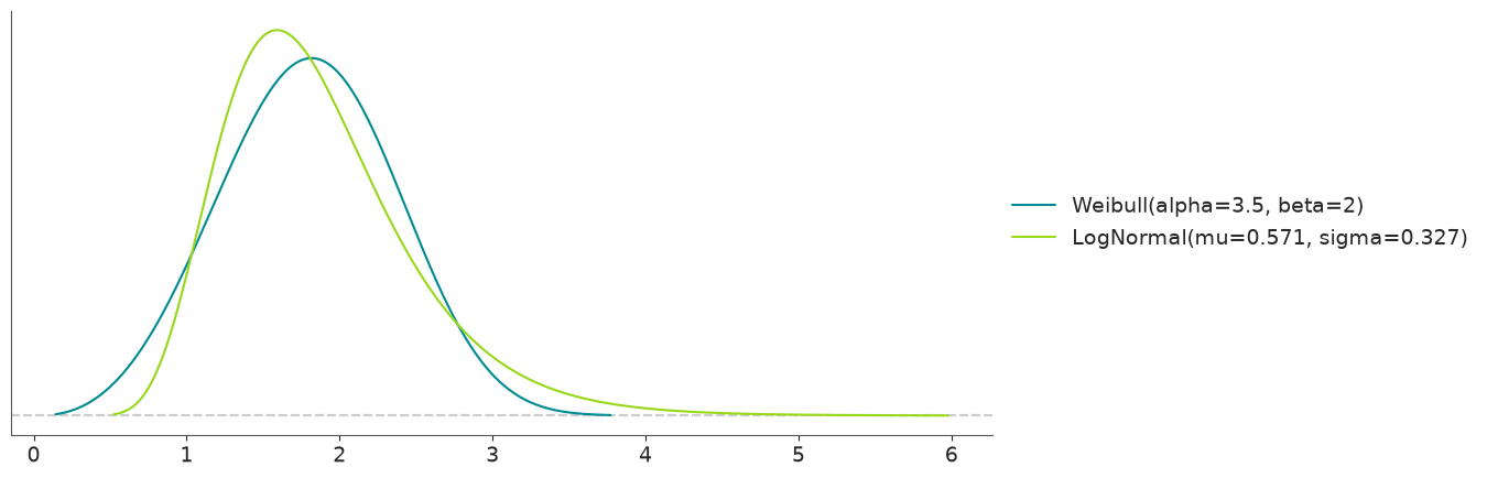
As with other functions we get a warning when the matching is worst than a threshold, so we can decide if the result is acceptable for our purposes.
The roulette method#
The roulette method allows us to find a prior distribution by drawing. The name roulette comes from the analogy that we are placing a limited set of chips where we think the mass of a distribution should be.
For this task, we are offered a grid of m equally sized bins covering the range of x. And we have to allocate a
total of n chips between the bins. In other words, we use a grid to draw a histogram and the function will try to tell
us what distribution, from a given pool of options, is a better fit for our drawing.
To use the Roulette we need to first call %matplotlib widget and have ipywidgets installed.
%matplotlib widget
result = pz.Roulette()
If you are unable to run the previous cell, you can get a glimpse of roulette from this gif
Once you have elicited the distribution you can call .dist attribute to get the distribution. In the following
example, it will be result.dist.
You can combine results for many independent “roulette sessions”. This could be useful to combine information from different sources, like different domain experts. Or even from a single person unable to pick a single option.
Anyway, let’s say that you run Roulette twice, for the first one you get result0 and for the second result1. Then
you can combine both solutions into a single one using
pz.combine_roulette([result0.inputs, result1.inputs], weights=[0.3, 0.7])
In this example, we are giving more weight (or importance) to the results from the second elicitation session. By default, the weights are equal.