Distributions#

`preliz.distributions.continuous`#

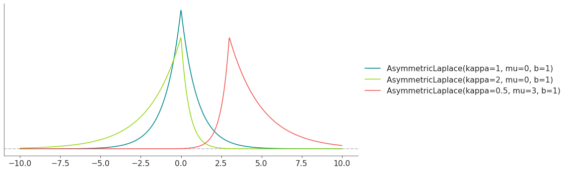
class preliz.distributions.asymmetric_laplace.AsymmetricLaplace(kappa=None, mu=None, b=None, q=None)[source]#

Asymmetric-Laplace distribution.

The pdf of this distribution is

\[\begin{split}{f(x|\\b,\kappa,\mu) = \left({\frac{\\b}{\kappa + 1/\kappa}}\right)\,e^{-(x-\mu)\\b\,s\kappa ^{s}}}\end{split}\]

where

\[s = sgn(x-\mu)\]

(Source code, png, hires.png, pdf)

Support	$x \in \mathbb{R}$
Mean	$\mu-\frac{\\\kappa-1/\kappa}b$
Variance	$\frac{1+\kappa^{4}}{b^2\kappa^2 }$

AsymmetricLaplace distribution has 2 alternative parametrizations. In terms of kappa, mu and b or q, mu and b.

The link between the 2 alternatives is given by

\[\kappa = \sqrt(\frac{q}{1-q})\]

Parameters:

kappa (float) – Symmetry parameter (kappa > 0).
mu (float) – Location parameter.
b (float) – Scale parameter (b > 0).
q (float) – Symmetry parameter (0 < q < 1).

cdf(x)[source]#

Cumulative distribution function.

Parameters:: x (array_like) – Values on which to evaluate the cdf

entropy()[source]#: Entropy.

eti(mass=None, fmt='.2f')#

Equal-tailed interval containing mass.

Parameters:

mass (float) – Probability mass in the interval. Defaults to None,
used. (which results in the value of rcParams["stats.ci_prob"] being)
fmt (str) – fmt used to represent results using f-string fmt for floats. Default to “.2f” i.e. 2 digits after the decimal point. Use “none” for no format.

hdi(mass=None, fmt='.2f')#

Highest density interval containing mass.

Parameters:

mass (float) – Probability mass in the interval. Defaults to None,
used. (which results in the value of rcParams["stats.ci_prob"] being)
fmt (str) – fmt used to represent results using f-string fmt for floats. Default to “.2f” i.e. 2 digits after the decimal point. Use “none” for no format.

isf(x)#

Inverse survival function (inverse of sf).

Parameters:: x (array_like) – Values on which to evaluate the inverse of the sf

kurtosis()[source]#: Excess kurtosis.

lmoment1()[source]#: L-moment1 (mean).

lmoment2()[source]#: L-moment2 (l-scale).

lmoment3()[source]#: L-moment3 (l-skewness). This the ratio of L-moment3 to L-moment2.

lmoment4()[source]#: L-moment4 (l-kurtosis). This the ratio of L-moment4 to L-moment2.

lmoments(types='1234')#

Compute L-moments of the distribution.

Parameters:: types (str) – The type of moments to compute. Default is ‘1234’ where ‘1’ = L-moment1 (mean), ‘2’ = L-moment2 (l-scale), ‘3’ = L-moment3 (l-skewness), and ‘4’ = L-moment4 (l-kurtosis). To compute the standard deviation use ‘d’ Valid combinations are any subset of ‘1234’.

logcdf(x)#

Log cumulative distribution function.

Parameters:: x (array_like) – Values on which to evaluate the logcdf

logpdf(x)[source]#

Log probability density/mass function.

Parameters:: x (array_like) – Values on which to evaluate the logpdf

logsf(x)#

Log survival function log(1 - cdf).

Parameters:: x (array_like) – Values on which to evaluate the logsf

mean()[source]#: Mean.

median()[source]#: Median.

mode()[source]#: Mode.

moments(types='mvsk')#

Compute moments of the distribution.

It can also return the standard deviation

Parameters:: types (str) – The type of moments to compute. Default is ‘mvsk’ where ‘m’ = mean, ‘v’ = variance, ‘s’ = skewness, and ‘k’ = kurtosis. To compute the standard deviation use ‘d’ Valid combinations are any subset of ‘mvdsk’.

pdf(x)[source]#

Probability density/mass function.

Parameters:: x (array_like) – Values on which to evaluate the pdf

plot_cdf(moments=None, pointinterval=False, interval=None, levels=None, support='restricted', legend='legend', figsize=None, ax=None, **kwargs)#

Plot the cumulative distribution function.

Parameters:

moments (str) – Compute moments. Use any combination of the strings m, d, v, s or k for the mean (μ), standard deviation (σ), variance (σ²), skew (γ) or kurtosis (κ) respectively. Other strings will be ignored. Defaults to None.
pointinterval (bool) – Whether to include a plot of the quantiles. Defaults to False. If True the default is to plot the median and two interquantiles ranges.
interval (str) – Type of interval. Available options are highest density interval “hdi” (default), equal tailed interval “eti” or intervals defined by arbitrary “quantiles”. Defaults to the value in rcParams[“stats.ci_kind”].
levels (list) – Mass of the intervals. For hdi or eti the number of elements should be 2 or 1. For quantiles the number of elements should be 5, 3, 1 or 0 (in this last case nothing will be plotted).
support (str:) – If full use the finite end-points to set the limits of the plot. For unbounded end-points or if restricted use the 0.001 and 0.999 quantiles to set the limits.
legend (str) – Whether to include a string with the distribution and its parameter as a "legend" a "title" or not include them None.
figsize (tuple) – Size of the figure
ax (matplotlib axes)
kwargs (keyword arguments) – Additional keyword arguments passed to matplotlib plot function. For example, color, alpha, linewidth, etc.

plot_interactive(kind='pdf', xy_lim='both', pointinterval=True, interval=None, levels=None, figsize=None)#

Interactive exploration of distributions parameters.

Parameters:

kind (str:) – Type of plot. Available options are pdf, cdf and ppf.
xy_lim (str or tuple) – Set the limits of the x-axis and/or y-axis. Defaults to “both”, the limits of both axis are fixed. Use “auto” for automatic rescaling of x-axis and y-axis. Or set them manually by passing a tuple of 4 elements, the first two for x-axis, the last two for y-axis. The tuple can have None.
pointinterval (bool) – Whether to include a plot of the quantiles. Defaults to False. If True the default is to plot the median and two interquantiles ranges.
interval (str) – Type of interval. Available options are highest density interval “hdi” (default), equal tailed interval “eti” or intervals defined by arbitrary “quantiles”. Defaults to the value in rcParams[“stats.ci_kind”].
levels (list) – Mass of the intervals. For hdi or eti the number of elements should be 2 or 1. For quantiles the number of elements should be 5, 3, 1 or 0 (in this last case nothing will be plotted).
figsize (tuple) – Size of the figure

plot_isf(moments=None, pointinterval=False, interval=None, levels=None, legend='legend', figsize=None, ax=None, **kwargs)#

Plot the inverse survival function.

Parameters:

moments (str) – Compute moments. Use any combination of the strings m, d, v, s or k for the mean (μ), standard deviation (σ), variance (σ²), skew (γ) or kurtosis (κ) respectively. Other strings will be ignored. Defaults to None.
pointinterval (bool) – Whether to include a plot of the quantiles. Defaults to False. If True the default is to plot the median and two interquantiles ranges.
interval (str) – Type of interval. Available options are highest density interval “hdi” (default), equal tailed interval “eti” or intervals defined by arbitrary “quantiles”. Defaults to the value in rcParams[“stats.ci_kind”].
levels (list) – Mass of the intervals. For hdi or eti the number of elements should be 2 or 1. For quantiles the number of elements should be 5, 3, 1 or 0 (in this last case nothing will be plotted).
legend (str) – Whether to include a string with the distribution and its parameter as a "legend" a "title" or not include them None.
figsize (tuple) – Size of the figure
ax (matplotlib axes)

plot_pdf(moments=None, pointinterval=False, interval=None, levels=None, support='restricted', baseline=True, legend='legend', figsize=None, ax=None, **kwargs)#

Plot the pdf (continuous) or pmf (discrete).

Parameters:

moments (str) – Compute moments. Use any combination of the strings m, d, v, s or k for the mean (μ), standard deviation (σ), variance (σ²), skew (γ) or kurtosis (κ) respectively. Other strings will be ignored. Defaults to None.
pointinterval (bool) – Whether to include a plot of the quantiles. Defaults to False. If True the default is to plot the median and two interquantiles ranges.
interval (str) – Type of interval. Available options are highest density interval “hdi” (default), equal tailed interval “eti” or intervals defined by arbitrary “quantiles”. Defaults to the value in rcParams[“stats.ci_kind”].
levels (list) – Mass of the intervals. For hdi or eti the number of elements should be 2 or 1. For quantiles the number of elements should be 5, 3, 1 or 0 (in this last case nothing will be plotted).
support (str:) – If full use the finite end-points to set the limits of the plot. For unbounded end-points or if restricted use the 0.001 and 0.999 quantiles to set the limits.
baseline (bool) – Whether to include a horizontal line at y=0.
legend (str) – Whether to include a string with the distribution and its parameter as a "legend" a "title" or not include them None.
figsize (tuple) – Size of the figure
ax (matplotlib axes)
kwargs (keyword arguments) – Additional keyword arguments passed to matplotlib plot function. For example, color, alpha, linewidth, etc.

plot_ppf(moments=None, pointinterval=False, interval=None, levels=None, legend='legend', figsize=None, ax=None, **kwargs)#

Plot the quantile function.

Parameters:

moments (str) – Compute moments. Use any combination of the strings m, d, v, s or k for the mean (μ), standard deviation (σ), variance (σ²), skew (γ) or kurtosis (κ) respectively. Other strings will be ignored. Defaults to None.
pointinterval (bool) – Whether to include a plot of the quantiles. Defaults to False. If True the default is to plot the median and two interquantiles ranges.
interval (str) – Type of interval. Available options are highest density interval “hdi” (default), equal tailed interval “eti” or intervals defined by arbitrary “quantiles”. Defaults to the value in rcParams[“stats.ci_kind”].
levels (list) – Mass of the intervals. For hdi or eti the number of elements should be 2 or 1. For quantiles the number of elements should be 5, 3, 1 or 0 (in this last case nothing will be plotted).
legend (str) – Whether to include a string with the distribution and its parameter as a "legend" a "title" or not include them None.
figsize (tuple) – Size of the figure
ax (matplotlib axes)

plot_sf(moments=None, pointinterval=False, interval=None, levels=None, support='restricted', legend='legend', figsize=None, ax=None, **kwargs)#

Plot the survival distribution function (1 - CDF).

Parameters:

moments (str) – Compute moments. Use any combination of the strings m, d, v, s or k for the mean (μ), standard deviation (σ), variance (σ²), skew (γ) or kurtosis (κ) respectively. Other strings will be ignored. Defaults to None.
pointinterval (bool) – Whether to include a plot of the quantiles. Defaults to False. If True the default is to plot the median and two interquantiles ranges.
interval (str) – Type of interval. Available options are highest density interval “hdi” (default), equal tailed interval “eti” or intervals defined by arbitrary “quantiles”. Defaults to the value in rcParams[“stats.ci_kind”].
levels (list) – Mass of the intervals. For hdi or eti the number of elements should be 2 or 1. For quantiles the number of elements should be 5, 3, 1 or 0 (in this last case nothing will be plotted).
support (str:) – If full use the finite end-points to set the limits of the plot. For unbounded end-points or if restricted use the 0.001 and 0.999 quantiles to set the limits.
legend (str) – Whether to include a string with the distribution and its parameter as a "legend" a "title" or not include them None.
figsize (tuple) – Size of the figure
ax (matplotlib axes)
kwargs (keyword arguments) – Additional keyword arguments passed to matplotlib plot function. For example, color, alpha, linewidth, etc.

ppf(q)[source]#

Percent point function (inverse of cdf).

Parameters:: x (array_like) – Values on which to evaluate the inverse of the cdf

rvs(size=None, random_state=None)[source]#

Random sample.

Parameters:

size (int or tuple of ints, optional) – Defining number of random variates. Defaults to 1.
random_state ({None, int, numpy.random.Generator, numpy.random.RandomState}) – Defaults to None

sf(x)#

Survival function (1 - cdf).

Parameters:: x (array_like) – Values on which to evaluate the sf

skewness()[source]#: Skewness.

std()[source]#: Standard deviation.

summary(mass=None, interval=None, fmt='.2f')#

Namedtuple with the mean, median, sd, and lower and upper bounds.

Parameters:

mass (float) – Probability mass for the equal-tailed interval. Defaults to None,
used. (which results in the value of rcParams["stats.ci_prob"] being)
interval (str or list-like) – Type of interval. Available options are highest density interval “hdi”, equal tailed interval “eti” or arbitrary interval defined by a list-like object with a pair of values. Defaults to the value in rcParams[“stats.ci_kind”].
fmt (str) – fmt used to represent results using f-string fmt for floats. Default to “.2f” i.e. 2 digits after the decimal point.

to_bambi(**kwargs)#

Convert the PreliZ distribution to a Bambi Prior.

kwargsPyMC distributions properties: kwargs are used to specify properties such as shape or dims

Return type:: Bambi Prior

to_pymc(name=None, **kwargs)#

Convert the PreliZ distribution to a PyMC distribution.

namestr: Name of PyMC distribution. Needed if inside Model context
kwargsPyMC distributions properties: kwargs are used to specify properties such as shape or dims

Return type:: PyMC distribution

var()[source]#: Variance.

xvals(support, n_points=None)#

Provide x values in the support of the distribution.

This is useful for example when plotting.

Parameters:

support (str) – Available options are “full” or “restricted”. If “full” the values will cover the entire support of the distribution if the boundary is finite, or the quantiles 0.0001 or 0.9999, if infinite. If “restricted” the values will cover the quantile 0.0001 to 0.9999.
n_points (int) – Number of values to return. Defaults to 1000 for continuous distributions and 200 for discrete ones. For discrete distributions the returned values may be fewer than n_points if the actual number of discrete values in the support of the distribution is smaller than n_points.

Beta distribution.

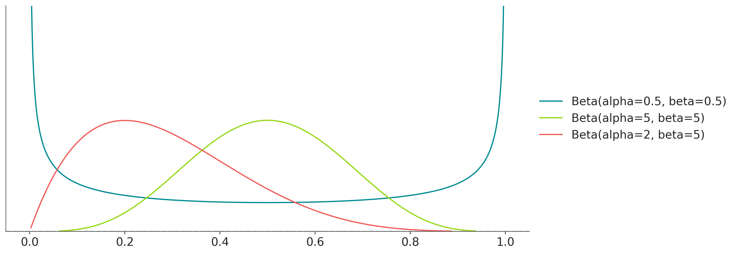
class preliz.distributions.beta.Beta(alpha=None, beta=None, mu=None, sigma=None, nu=None)[source]#

Beta distribution.

The pdf of this distribution is

\[f(x \mid \alpha, \beta) = \frac{x^{\alpha - 1} (1 - x)^{\beta - 1}}{B(\alpha, \beta)}\]

(Source code, png, hires.png, pdf)

Support	$x \in (0, 1)$
Mean	$\dfrac{\alpha}{\alpha + \beta}$
Variance	$\dfrac{\alpha \beta}{(\alpha+\beta)^2(\alpha+\beta+1)}$

Beta distribution has 3 alternative parameterizations. In terms of alpha and beta, mean and sigma (standard deviation) or mean and nu (concentration).

The link between the 3 alternatives is given by

\[ \begin{align}\begin{aligned}\begin{split}\alpha &= \mu \nu \\ \beta &= (1 - \mu) \nu\end{split}\\\text{where } \nu = \frac{\mu(1-\mu)}{\sigma^2} - 1\end{aligned}\end{align} \]

Parameters:

alpha (float) – alpha > 0
beta (float) – beta > 0
mu (float) – mean (0 < mu < 1).
sigma (float) – standard deviation (sigma < sqrt(mu * (1 - mu))).
nu (float) – concentration > 0

cdf(x)[source]#

Cumulative distribution function.

Parameters:: x (array_like) – Values on which to evaluate the cdf

entropy()[source]#: Entropy.

eti(mass=None, fmt='.2f')#

Equal-tailed interval containing mass.

Parameters:

mass (float) – Probability mass in the interval. Defaults to None,
used. (which results in the value of rcParams["stats.ci_prob"] being)
fmt (str) – fmt used to represent results using f-string fmt for floats. Default to “.2f” i.e. 2 digits after the decimal point. Use “none” for no format.

hdi(mass=None, fmt='.2f')#

Highest density interval containing mass.

Parameters:

mass (float) – Probability mass in the interval. Defaults to None,
used. (which results in the value of rcParams["stats.ci_prob"] being)
fmt (str) – fmt used to represent results using f-string fmt for floats. Default to “.2f” i.e. 2 digits after the decimal point. Use “none” for no format.

isf(q)[source]#

Inverse survival function (inverse of sf).

Parameters:: x (array_like) – Values on which to evaluate the inverse of the sf

kurtosis()[source]#: Excess kurtosis.

lmoment1()[source]#: L-moment1 (mean).

lmoment2()[source]#: L-moment2 (l-scale).

lmoment3()[source]#: L-moment3 (l-skewness). This the ratio of L-moment3 to L-moment2.

lmoment4()[source]#: L-moment4 (l-kurtosis). This the ratio of L-moment4 to L-moment2.

lmoments(types='1234')#

Compute L-moments of the distribution.

Parameters:: types (str) – The type of moments to compute. Default is ‘1234’ where ‘1’ = L-moment1 (mean), ‘2’ = L-moment2 (l-scale), ‘3’ = L-moment3 (l-skewness), and ‘4’ = L-moment4 (l-kurtosis). To compute the standard deviation use ‘d’ Valid combinations are any subset of ‘1234’.

logcdf(x)[source]#

Log cumulative distribution function.

Parameters:: x (array_like) – Values on which to evaluate the logcdf

logpdf(x)[source]#

Log probability density/mass function.

Parameters:: x (array_like) – Values on which to evaluate the logpdf

logsf(x)[source]#

Log survival function log(1 - cdf).

Parameters:: x (array_like) – Values on which to evaluate the logsf

mean()[source]#: Mean.

median()[source]#: Median.

mode()[source]#: Mode.

moments(types='mvsk')#

Compute moments of the distribution.

It can also return the standard deviation

Parameters:: types (str) – The type of moments to compute. Default is ‘mvsk’ where ‘m’ = mean, ‘v’ = variance, ‘s’ = skewness, and ‘k’ = kurtosis. To compute the standard deviation use ‘d’ Valid combinations are any subset of ‘mvdsk’.

pdf(x)[source]#

Probability density/mass function.

Parameters:: x (array_like) – Values on which to evaluate the pdf

plot_cdf(moments=None, pointinterval=False, interval=None, levels=None, support='restricted', legend='legend', figsize=None, ax=None, **kwargs)#

Plot the cumulative distribution function.

Parameters:

moments (str) – Compute moments. Use any combination of the strings m, d, v, s or k for the mean (μ), standard deviation (σ), variance (σ²), skew (γ) or kurtosis (κ) respectively. Other strings will be ignored. Defaults to None.
pointinterval (bool) – Whether to include a plot of the quantiles. Defaults to False. If True the default is to plot the median and two interquantiles ranges.
interval (str) – Type of interval. Available options are highest density interval “hdi” (default), equal tailed interval “eti” or intervals defined by arbitrary “quantiles”. Defaults to the value in rcParams[“stats.ci_kind”].
levels (list) – Mass of the intervals. For hdi or eti the number of elements should be 2 or 1. For quantiles the number of elements should be 5, 3, 1 or 0 (in this last case nothing will be plotted).
support (str:) – If full use the finite end-points to set the limits of the plot. For unbounded end-points or if restricted use the 0.001 and 0.999 quantiles to set the limits.
legend (str) – Whether to include a string with the distribution and its parameter as a "legend" a "title" or not include them None.
figsize (tuple) – Size of the figure
ax (matplotlib axes)
kwargs (keyword arguments) – Additional keyword arguments passed to matplotlib plot function. For example, color, alpha, linewidth, etc.

plot_interactive(kind='pdf', xy_lim='both', pointinterval=True, interval=None, levels=None, figsize=None)#

Interactive exploration of distributions parameters.

Parameters:

kind (str:) – Type of plot. Available options are pdf, cdf and ppf.
xy_lim (str or tuple) – Set the limits of the x-axis and/or y-axis. Defaults to “both”, the limits of both axis are fixed. Use “auto” for automatic rescaling of x-axis and y-axis. Or set them manually by passing a tuple of 4 elements, the first two for x-axis, the last two for y-axis. The tuple can have None.
pointinterval (bool) – Whether to include a plot of the quantiles. Defaults to False. If True the default is to plot the median and two interquantiles ranges.
interval (str) – Type of interval. Available options are highest density interval “hdi” (default), equal tailed interval “eti” or intervals defined by arbitrary “quantiles”. Defaults to the value in rcParams[“stats.ci_kind”].
levels (list) – Mass of the intervals. For hdi or eti the number of elements should be 2 or 1. For quantiles the number of elements should be 5, 3, 1 or 0 (in this last case nothing will be plotted).
figsize (tuple) – Size of the figure

plot_isf(moments=None, pointinterval=False, interval=None, levels=None, legend='legend', figsize=None, ax=None, **kwargs)#

Plot the inverse survival function.

Parameters:

moments (str) – Compute moments. Use any combination of the strings m, d, v, s or k for the mean (μ), standard deviation (σ), variance (σ²), skew (γ) or kurtosis (κ) respectively. Other strings will be ignored. Defaults to None.
pointinterval (bool) – Whether to include a plot of the quantiles. Defaults to False. If True the default is to plot the median and two interquantiles ranges.
interval (str) – Type of interval. Available options are highest density interval “hdi” (default), equal tailed interval “eti” or intervals defined by arbitrary “quantiles”. Defaults to the value in rcParams[“stats.ci_kind”].
levels (list) – Mass of the intervals. For hdi or eti the number of elements should be 2 or 1. For quantiles the number of elements should be 5, 3, 1 or 0 (in this last case nothing will be plotted).
legend (str) – Whether to include a string with the distribution and its parameter as a "legend" a "title" or not include them None.
figsize (tuple) – Size of the figure
ax (matplotlib axes)

plot_pdf(moments=None, pointinterval=False, interval=None, levels=None, support='restricted', baseline=True, legend='legend', figsize=None, ax=None, **kwargs)#

Plot the pdf (continuous) or pmf (discrete).

Parameters:

moments (str) – Compute moments. Use any combination of the strings m, d, v, s or k for the mean (μ), standard deviation (σ), variance (σ²), skew (γ) or kurtosis (κ) respectively. Other strings will be ignored. Defaults to None.
pointinterval (bool) – Whether to include a plot of the quantiles. Defaults to False. If True the default is to plot the median and two interquantiles ranges.
interval (str) – Type of interval. Available options are highest density interval “hdi” (default), equal tailed interval “eti” or intervals defined by arbitrary “quantiles”. Defaults to the value in rcParams[“stats.ci_kind”].
levels (list) – Mass of the intervals. For hdi or eti the number of elements should be 2 or 1. For quantiles the number of elements should be 5, 3, 1 or 0 (in this last case nothing will be plotted).
support (str:) – If full use the finite end-points to set the limits of the plot. For unbounded end-points or if restricted use the 0.001 and 0.999 quantiles to set the limits.
baseline (bool) – Whether to include a horizontal line at y=0.
legend (str) – Whether to include a string with the distribution and its parameter as a "legend" a "title" or not include them None.
figsize (tuple) – Size of the figure
ax (matplotlib axes)
kwargs (keyword arguments) – Additional keyword arguments passed to matplotlib plot function. For example, color, alpha, linewidth, etc.

plot_ppf(moments=None, pointinterval=False, interval=None, levels=None, legend='legend', figsize=None, ax=None, **kwargs)#

Plot the quantile function.

Parameters:

moments (str) – Compute moments. Use any combination of the strings m, d, v, s or k for the mean (μ), standard deviation (σ), variance (σ²), skew (γ) or kurtosis (κ) respectively. Other strings will be ignored. Defaults to None.
pointinterval (bool) – Whether to include a plot of the quantiles. Defaults to False. If True the default is to plot the median and two interquantiles ranges.
interval (str) – Type of interval. Available options are highest density interval “hdi” (default), equal tailed interval “eti” or intervals defined by arbitrary “quantiles”. Defaults to the value in rcParams[“stats.ci_kind”].
levels (list) – Mass of the intervals. For hdi or eti the number of elements should be 2 or 1. For quantiles the number of elements should be 5, 3, 1 or 0 (in this last case nothing will be plotted).
legend (str) – Whether to include a string with the distribution and its parameter as a "legend" a "title" or not include them None.
figsize (tuple) – Size of the figure
ax (matplotlib axes)

plot_sf(moments=None, pointinterval=False, interval=None, levels=None, support='restricted', legend='legend', figsize=None, ax=None, **kwargs)#

Plot the survival distribution function (1 - CDF).

Parameters:

moments (str) – Compute moments. Use any combination of the strings m, d, v, s or k for the mean (μ), standard deviation (σ), variance (σ²), skew (γ) or kurtosis (κ) respectively. Other strings will be ignored. Defaults to None.
pointinterval (bool) – Whether to include a plot of the quantiles. Defaults to False. If True the default is to plot the median and two interquantiles ranges.
interval (str) – Type of interval. Available options are highest density interval “hdi” (default), equal tailed interval “eti” or intervals defined by arbitrary “quantiles”. Defaults to the value in rcParams[“stats.ci_kind”].
levels (list) – Mass of the intervals. For hdi or eti the number of elements should be 2 or 1. For quantiles the number of elements should be 5, 3, 1 or 0 (in this last case nothing will be plotted).
support (str:) – If full use the finite end-points to set the limits of the plot. For unbounded end-points or if restricted use the 0.001 and 0.999 quantiles to set the limits.
legend (str) – Whether to include a string with the distribution and its parameter as a "legend" a "title" or not include them None.
figsize (tuple) – Size of the figure
ax (matplotlib axes)
kwargs (keyword arguments) – Additional keyword arguments passed to matplotlib plot function. For example, color, alpha, linewidth, etc.

ppf(q)[source]#

Percent point function (inverse of cdf).

Parameters:: x (array_like) – Values on which to evaluate the inverse of the cdf

rvs(size=None, random_state=None)[source]#

Random sample.

Parameters:

size (int or tuple of ints, optional) – Defining number of random variates. Defaults to 1.
random_state ({None, int, numpy.random.Generator, numpy.random.RandomState}) – Defaults to None

sf(x)[source]#

Survival function (1 - cdf).

Parameters:: x (array_like) – Values on which to evaluate the sf

skewness()[source]#: Skewness.

std()[source]#: Standard deviation.

summary(mass=None, interval=None, fmt='.2f')#

Namedtuple with the mean, median, sd, and lower and upper bounds.

Parameters:

mass (float) – Probability mass for the equal-tailed interval. Defaults to None,
used. (which results in the value of rcParams["stats.ci_prob"] being)
interval (str or list-like) – Type of interval. Available options are highest density interval “hdi”, equal tailed interval “eti” or arbitrary interval defined by a list-like object with a pair of values. Defaults to the value in rcParams[“stats.ci_kind”].
fmt (str) – fmt used to represent results using f-string fmt for floats. Default to “.2f” i.e. 2 digits after the decimal point.

to_bambi(**kwargs)#

Convert the PreliZ distribution to a Bambi Prior.

kwargsPyMC distributions properties: kwargs are used to specify properties such as shape or dims

Return type:: Bambi Prior

to_pymc(name=None, **kwargs)#

Convert the PreliZ distribution to a PyMC distribution.

namestr: Name of PyMC distribution. Needed if inside Model context
kwargsPyMC distributions properties: kwargs are used to specify properties such as shape or dims

Return type:: PyMC distribution

var()[source]#: Variance.

xvals(support, n_points=None)#

Provide x values in the support of the distribution.

This is useful for example when plotting.

Parameters:

support (str) – Available options are “full” or “restricted”. If “full” the values will cover the entire support of the distribution if the boundary is finite, or the quantiles 0.0001 or 0.9999, if infinite. If “restricted” the values will cover the quantile 0.0001 to 0.9999.
n_points (int) – Number of values to return. Defaults to 1000 for continuous distributions and 200 for discrete ones. For discrete distributions the returned values may be fewer than n_points if the actual number of discrete values in the support of the distribution is smaller than n_points.

BetaScaled distribution.

class preliz.distributions.betascaled.BetaScaled(alpha=None, beta=None, lower=0, upper=1)[source]#

Scaled Beta distribution.

The pdf of this distribution is

\[f(x \mid \alpha, \beta) = \frac{(x-\text{lower})^{\alpha - 1} (\text{upper} - x)^{\beta - 1}} {(\text{upper}-\text{lower})^{\alpha+\beta-1} B(\alpha, \beta)}\]

(Source code, png, hires.png, pdf)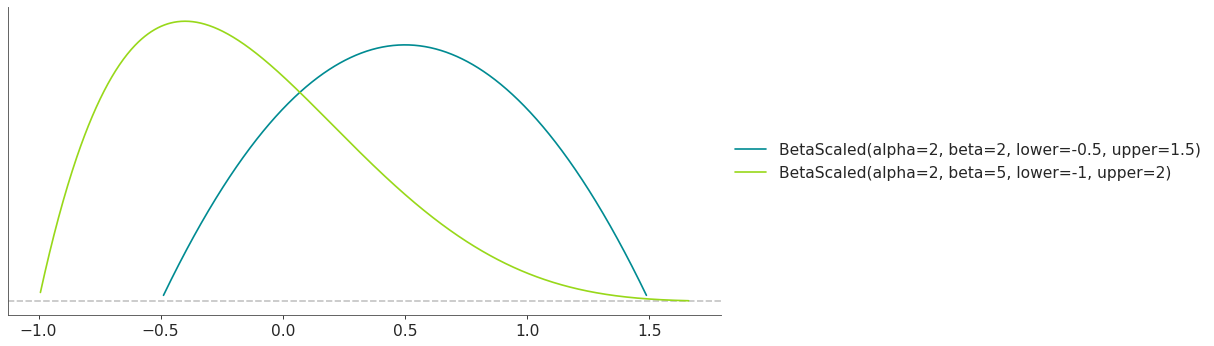

Support	$x \in (lower, upper)$
Mean	$\dfrac{\alpha}{\alpha + \beta} (upper-lower) + lower$
Variance	$\dfrac{\alpha \beta}{(\alpha+\beta)^2(\alpha+\beta+1)} (upper-lower)$

Parameters:

alpha (float) – alpha > 0
beta (float) – beta > 0
lower (float) – Lower limit.
upper (float) – Upper limit (upper > lower).

cdf(x)[source]#

Cumulative distribution function.

Parameters:: x (array_like) – Values on which to evaluate the cdf

entropy()[source]#: Entropy.

eti(mass=None, fmt='.2f')#

Equal-tailed interval containing mass.

Parameters:

mass (float) – Probability mass in the interval. Defaults to None,
used. (which results in the value of rcParams["stats.ci_prob"] being)
fmt (str) – fmt used to represent results using f-string fmt for floats. Default to “.2f” i.e. 2 digits after the decimal point. Use “none” for no format.

hdi(mass=None, fmt='.2f')#

Highest density interval containing mass.

Parameters:

mass (float) – Probability mass in the interval. Defaults to None,
used. (which results in the value of rcParams["stats.ci_prob"] being)
fmt (str) – fmt used to represent results using f-string fmt for floats. Default to “.2f” i.e. 2 digits after the decimal point. Use “none” for no format.

isf(q)[source]#

Inverse survival function (inverse of sf).

Parameters:: x (array_like) – Values on which to evaluate the inverse of the sf

kurtosis()[source]#: Excess kurtosis.

lmoment1()[source]#: L-moment1 (mean).

lmoment2()[source]#: L-moment2 (l-scale).

lmoment3()[source]#: L-moment3 (l-skewness). This the ratio of L-moment3 to L-moment2.

lmoment4()[source]#: L-moment4 (l-kurtosis). This the ratio of L-moment4 to L-moment2.

lmoments(types='1234')#

Compute L-moments of the distribution.

Parameters:: types (str) – The type of moments to compute. Default is ‘1234’ where ‘1’ = L-moment1 (mean), ‘2’ = L-moment2 (l-scale), ‘3’ = L-moment3 (l-skewness), and ‘4’ = L-moment4 (l-kurtosis). To compute the standard deviation use ‘d’ Valid combinations are any subset of ‘1234’.

logcdf(x)[source]#

Log cumulative distribution function.

Parameters:: x (array_like) – Values on which to evaluate the logcdf

logpdf(x)[source]#

Log probability density/mass function.

Parameters:: x (array_like) – Values on which to evaluate the logpdf

logsf(x)[source]#

Log survival function log(1 - cdf).

Parameters:: x (array_like) – Values on which to evaluate the logsf

mean()[source]#: Mean.

median()[source]#: Median.

mode()[source]#: Mode.

moments(types='mvsk')#

Compute moments of the distribution.

It can also return the standard deviation

Parameters:: types (str) – The type of moments to compute. Default is ‘mvsk’ where ‘m’ = mean, ‘v’ = variance, ‘s’ = skewness, and ‘k’ = kurtosis. To compute the standard deviation use ‘d’ Valid combinations are any subset of ‘mvdsk’.

pdf(x)[source]#

Probability density/mass function.

Parameters:: x (array_like) – Values on which to evaluate the pdf

plot_cdf(moments=None, pointinterval=False, interval=None, levels=None, support='restricted', legend='legend', figsize=None, ax=None, **kwargs)#

Plot the cumulative distribution function.

Parameters:

moments (str) – Compute moments. Use any combination of the strings m, d, v, s or k for the mean (μ), standard deviation (σ), variance (σ²), skew (γ) or kurtosis (κ) respectively. Other strings will be ignored. Defaults to None.
pointinterval (bool) – Whether to include a plot of the quantiles. Defaults to False. If True the default is to plot the median and two interquantiles ranges.
interval (str) – Type of interval. Available options are highest density interval “hdi” (default), equal tailed interval “eti” or intervals defined by arbitrary “quantiles”. Defaults to the value in rcParams[“stats.ci_kind”].
levels (list) – Mass of the intervals. For hdi or eti the number of elements should be 2 or 1. For quantiles the number of elements should be 5, 3, 1 or 0 (in this last case nothing will be plotted).
support (str:) – If full use the finite end-points to set the limits of the plot. For unbounded end-points or if restricted use the 0.001 and 0.999 quantiles to set the limits.
legend (str) – Whether to include a string with the distribution and its parameter as a "legend" a "title" or not include them None.
figsize (tuple) – Size of the figure
ax (matplotlib axes)
kwargs (keyword arguments) – Additional keyword arguments passed to matplotlib plot function. For example, color, alpha, linewidth, etc.

plot_interactive(kind='pdf', xy_lim='both', pointinterval=True, interval=None, levels=None, figsize=None)#

Interactive exploration of distributions parameters.

Parameters:

kind (str:) – Type of plot. Available options are pdf, cdf and ppf.
xy_lim (str or tuple) – Set the limits of the x-axis and/or y-axis. Defaults to “both”, the limits of both axis are fixed. Use “auto” for automatic rescaling of x-axis and y-axis. Or set them manually by passing a tuple of 4 elements, the first two for x-axis, the last two for y-axis. The tuple can have None.
pointinterval (bool) – Whether to include a plot of the quantiles. Defaults to False. If True the default is to plot the median and two interquantiles ranges.
interval (str) – Type of interval. Available options are highest density interval “hdi” (default), equal tailed interval “eti” or intervals defined by arbitrary “quantiles”. Defaults to the value in rcParams[“stats.ci_kind”].
levels (list) – Mass of the intervals. For hdi or eti the number of elements should be 2 or 1. For quantiles the number of elements should be 5, 3, 1 or 0 (in this last case nothing will be plotted).
figsize (tuple) – Size of the figure

plot_isf(moments=None, pointinterval=False, interval=None, levels=None, legend='legend', figsize=None, ax=None, **kwargs)#

Plot the inverse survival function.

Parameters:

moments (str) – Compute moments. Use any combination of the strings m, d, v, s or k for the mean (μ), standard deviation (σ), variance (σ²), skew (γ) or kurtosis (κ) respectively. Other strings will be ignored. Defaults to None.
pointinterval (bool) – Whether to include a plot of the quantiles. Defaults to False. If True the default is to plot the median and two interquantiles ranges.
interval (str) – Type of interval. Available options are highest density interval “hdi” (default), equal tailed interval “eti” or intervals defined by arbitrary “quantiles”. Defaults to the value in rcParams[“stats.ci_kind”].
levels (list) – Mass of the intervals. For hdi or eti the number of elements should be 2 or 1. For quantiles the number of elements should be 5, 3, 1 or 0 (in this last case nothing will be plotted).
legend (str) – Whether to include a string with the distribution and its parameter as a "legend" a "title" or not include them None.
figsize (tuple) – Size of the figure
ax (matplotlib axes)

plot_pdf(moments=None, pointinterval=False, interval=None, levels=None, support='restricted', baseline=True, legend='legend', figsize=None, ax=None, **kwargs)#

Plot the pdf (continuous) or pmf (discrete).

Parameters:

moments (str) – Compute moments. Use any combination of the strings m, d, v, s or k for the mean (μ), standard deviation (σ), variance (σ²), skew (γ) or kurtosis (κ) respectively. Other strings will be ignored. Defaults to None.
pointinterval (bool) – Whether to include a plot of the quantiles. Defaults to False. If True the default is to plot the median and two interquantiles ranges.
interval (str) – Type of interval. Available options are highest density interval “hdi” (default), equal tailed interval “eti” or intervals defined by arbitrary “quantiles”. Defaults to the value in rcParams[“stats.ci_kind”].
levels (list) – Mass of the intervals. For hdi or eti the number of elements should be 2 or 1. For quantiles the number of elements should be 5, 3, 1 or 0 (in this last case nothing will be plotted).
support (str:) – If full use the finite end-points to set the limits of the plot. For unbounded end-points or if restricted use the 0.001 and 0.999 quantiles to set the limits.
baseline (bool) – Whether to include a horizontal line at y=0.
legend (str) – Whether to include a string with the distribution and its parameter as a "legend" a "title" or not include them None.
figsize (tuple) – Size of the figure
ax (matplotlib axes)
kwargs (keyword arguments) – Additional keyword arguments passed to matplotlib plot function. For example, color, alpha, linewidth, etc.

plot_ppf(moments=None, pointinterval=False, interval=None, levels=None, legend='legend', figsize=None, ax=None, **kwargs)#

Plot the quantile function.

Parameters:

moments (str) – Compute moments. Use any combination of the strings m, d, v, s or k for the mean (μ), standard deviation (σ), variance (σ²), skew (γ) or kurtosis (κ) respectively. Other strings will be ignored. Defaults to None.
pointinterval (bool) – Whether to include a plot of the quantiles. Defaults to False. If True the default is to plot the median and two interquantiles ranges.
interval (str) – Type of interval. Available options are highest density interval “hdi” (default), equal tailed interval “eti” or intervals defined by arbitrary “quantiles”. Defaults to the value in rcParams[“stats.ci_kind”].
levels (list) – Mass of the intervals. For hdi or eti the number of elements should be 2 or 1. For quantiles the number of elements should be 5, 3, 1 or 0 (in this last case nothing will be plotted).
legend (str) – Whether to include a string with the distribution and its parameter as a "legend" a "title" or not include them None.
figsize (tuple) – Size of the figure
ax (matplotlib axes)

plot_sf(moments=None, pointinterval=False, interval=None, levels=None, support='restricted', legend='legend', figsize=None, ax=None, **kwargs)#

Plot the survival distribution function (1 - CDF).

Parameters:

moments (str) – Compute moments. Use any combination of the strings m, d, v, s or k for the mean (μ), standard deviation (σ), variance (σ²), skew (γ) or kurtosis (κ) respectively. Other strings will be ignored. Defaults to None.
pointinterval (bool) – Whether to include a plot of the quantiles. Defaults to False. If True the default is to plot the median and two interquantiles ranges.
interval (str) – Type of interval. Available options are highest density interval “hdi” (default), equal tailed interval “eti” or intervals defined by arbitrary “quantiles”. Defaults to the value in rcParams[“stats.ci_kind”].
levels (list) – Mass of the intervals. For hdi or eti the number of elements should be 2 or 1. For quantiles the number of elements should be 5, 3, 1 or 0 (in this last case nothing will be plotted).
support (str:) – If full use the finite end-points to set the limits of the plot. For unbounded end-points or if restricted use the 0.001 and 0.999 quantiles to set the limits.
legend (str) – Whether to include a string with the distribution and its parameter as a "legend" a "title" or not include them None.
figsize (tuple) – Size of the figure
ax (matplotlib axes)
kwargs (keyword arguments) – Additional keyword arguments passed to matplotlib plot function. For example, color, alpha, linewidth, etc.

ppf(q)[source]#

Percent point function (inverse of cdf).

Parameters:: x (array_like) – Values on which to evaluate the inverse of the cdf

rvs(size=None, random_state=None)[source]#

Random sample.

Parameters:

size (int or tuple of ints, optional) – Defining number of random variates. Defaults to 1.
random_state ({None, int, numpy.random.Generator, numpy.random.RandomState}) – Defaults to None

sf(x)[source]#

Survival function (1 - cdf).

Parameters:: x (array_like) – Values on which to evaluate the sf

skewness()[source]#: Skewness.

std()[source]#: Standard deviation.

summary(mass=None, interval=None, fmt='.2f')#

Namedtuple with the mean, median, sd, and lower and upper bounds.

Parameters:

mass (float) – Probability mass for the equal-tailed interval. Defaults to None,
used. (which results in the value of rcParams["stats.ci_prob"] being)
interval (str or list-like) – Type of interval. Available options are highest density interval “hdi”, equal tailed interval “eti” or arbitrary interval defined by a list-like object with a pair of values. Defaults to the value in rcParams[“stats.ci_kind”].
fmt (str) – fmt used to represent results using f-string fmt for floats. Default to “.2f” i.e. 2 digits after the decimal point.

to_bambi(**kwargs)#

Convert the PreliZ distribution to a Bambi Prior.

kwargsPyMC distributions properties: kwargs are used to specify properties such as shape or dims

Return type:: Bambi Prior

to_pymc(name=None, **kwargs)#

Convert the PreliZ distribution to a PyMC distribution.

namestr: Name of PyMC distribution. Needed if inside Model context
kwargsPyMC distributions properties: kwargs are used to specify properties such as shape or dims

Return type:: PyMC distribution

var()[source]#: Variance.

xvals(support, n_points=None)#

Provide x values in the support of the distribution.

This is useful for example when plotting.

Parameters:

support (str) – Available options are “full” or “restricted”. If “full” the values will cover the entire support of the distribution if the boundary is finite, or the quantiles 0.0001 or 0.9999, if infinite. If “restricted” the values will cover the quantile 0.0001 to 0.9999.
n_points (int) – Number of values to return. Defaults to 1000 for continuous distributions and 200 for discrete ones. For discrete distributions the returned values may be fewer than n_points if the actual number of discrete values in the support of the distribution is smaller than n_points.

class preliz.distributions.cauchy.Cauchy(alpha=None, beta=None)[source]#

Cauchy Distribution.

The pdf of this distribution is

\[f(x \mid \alpha, \beta) = \frac{1}{\pi \beta [1 + (\frac{x-\alpha}{\beta})^2]}\]

(Source code, png, hires.png, pdf)

Support	$x \in \mathbb{R}$
Mean	undefined
Variance	undefined

Parameters:

alpha (float) – Location parameter.
beta (float) – Scale parameter > 0.

cdf(x)[source]#

Cumulative distribution function.

Parameters:: x (array_like) – Values on which to evaluate the cdf

entropy()[source]#: Entropy.

eti(mass=None, fmt='.2f')#

Equal-tailed interval containing mass.

Parameters:

mass (float) – Probability mass in the interval. Defaults to None,
used. (which results in the value of rcParams["stats.ci_prob"] being)
fmt (str) – fmt used to represent results using f-string fmt for floats. Default to “.2f” i.e. 2 digits after the decimal point. Use “none” for no format.

hdi(mass=None, fmt='.2f')#

Highest density interval containing mass.

Parameters:

mass (float) – Probability mass in the interval. Defaults to None,
used. (which results in the value of rcParams["stats.ci_prob"] being)
fmt (str) – fmt used to represent results using f-string fmt for floats. Default to “.2f” i.e. 2 digits after the decimal point. Use “none” for no format.

isf(x)#

Inverse survival function (inverse of sf).

Parameters:: x (array_like) – Values on which to evaluate the inverse of the sf

kurtosis()[source]#: Excess kurtosis.

lmoment1()[source]#: L-moment1 (mean).

lmoment2()[source]#: L-moment2 (l-scale).

lmoment3()[source]#: L-moment3 (l-skewness). This the ratio of L-moment3 to L-moment2.

lmoment4()[source]#: L-moment4 (l-kurtosis). This the ratio of L-moment4 to L-moment2.

lmoments(types='1234')#

Compute L-moments of the distribution.

Parameters:: types (str) – The type of moments to compute. Default is ‘1234’ where ‘1’ = L-moment1 (mean), ‘2’ = L-moment2 (l-scale), ‘3’ = L-moment3 (l-skewness), and ‘4’ = L-moment4 (l-kurtosis). To compute the standard deviation use ‘d’ Valid combinations are any subset of ‘1234’.

logcdf(x)[source]#

Log cumulative distribution function.

Parameters:: x (array_like) – Values on which to evaluate the logcdf

logpdf(x)[source]#

Log probability density/mass function.

Parameters:: x (array_like) – Values on which to evaluate the logpdf

logsf(x)[source]#

Log survival function log(1 - cdf).

Parameters:: x (array_like) – Values on which to evaluate the logsf

mean()[source]#: Mean.

median()[source]#: Median.

mode()[source]#: Mode.

moments(types='mvsk')#

Compute moments of the distribution.

It can also return the standard deviation

Parameters:: types (str) – The type of moments to compute. Default is ‘mvsk’ where ‘m’ = mean, ‘v’ = variance, ‘s’ = skewness, and ‘k’ = kurtosis. To compute the standard deviation use ‘d’ Valid combinations are any subset of ‘mvdsk’.

pdf(x)[source]#

Probability density/mass function.

Parameters:: x (array_like) – Values on which to evaluate the pdf

plot_cdf(moments=None, pointinterval=False, interval=None, levels=None, support='restricted', legend='legend', figsize=None, ax=None, **kwargs)#

Plot the cumulative distribution function.

Parameters:

moments (str) – Compute moments. Use any combination of the strings m, d, v, s or k for the mean (μ), standard deviation (σ), variance (σ²), skew (γ) or kurtosis (κ) respectively. Other strings will be ignored. Defaults to None.
pointinterval (bool) – Whether to include a plot of the quantiles. Defaults to False. If True the default is to plot the median and two interquantiles ranges.
interval (str) – Type of interval. Available options are highest density interval “hdi” (default), equal tailed interval “eti” or intervals defined by arbitrary “quantiles”. Defaults to the value in rcParams[“stats.ci_kind”].
levels (list) – Mass of the intervals. For hdi or eti the number of elements should be 2 or 1. For quantiles the number of elements should be 5, 3, 1 or 0 (in this last case nothing will be plotted).
support (str:) – If full use the finite end-points to set the limits of the plot. For unbounded end-points or if restricted use the 0.001 and 0.999 quantiles to set the limits.
legend (str) – Whether to include a string with the distribution and its parameter as a "legend" a "title" or not include them None.
figsize (tuple) – Size of the figure
ax (matplotlib axes)
kwargs (keyword arguments) – Additional keyword arguments passed to matplotlib plot function. For example, color, alpha, linewidth, etc.

plot_interactive(kind='pdf', xy_lim='both', pointinterval=True, interval=None, levels=None, figsize=None)#

Interactive exploration of distributions parameters.

Parameters:

kind (str:) – Type of plot. Available options are pdf, cdf and ppf.
xy_lim (str or tuple) – Set the limits of the x-axis and/or y-axis. Defaults to “both”, the limits of both axis are fixed. Use “auto” for automatic rescaling of x-axis and y-axis. Or set them manually by passing a tuple of 4 elements, the first two for x-axis, the last two for y-axis. The tuple can have None.
pointinterval (bool) – Whether to include a plot of the quantiles. Defaults to False. If True the default is to plot the median and two interquantiles ranges.
interval (str) – Type of interval. Available options are highest density interval “hdi” (default), equal tailed interval “eti” or intervals defined by arbitrary “quantiles”. Defaults to the value in rcParams[“stats.ci_kind”].
levels (list) – Mass of the intervals. For hdi or eti the number of elements should be 2 or 1. For quantiles the number of elements should be 5, 3, 1 or 0 (in this last case nothing will be plotted).
figsize (tuple) – Size of the figure

plot_isf(moments=None, pointinterval=False, interval=None, levels=None, legend='legend', figsize=None, ax=None, **kwargs)#

Plot the inverse survival function.

Parameters:

moments (str) – Compute moments. Use any combination of the strings m, d, v, s or k for the mean (μ), standard deviation (σ), variance (σ²), skew (γ) or kurtosis (κ) respectively. Other strings will be ignored. Defaults to None.
pointinterval (bool) – Whether to include a plot of the quantiles. Defaults to False. If True the default is to plot the median and two interquantiles ranges.
interval (str) – Type of interval. Available options are highest density interval “hdi” (default), equal tailed interval “eti” or intervals defined by arbitrary “quantiles”. Defaults to the value in rcParams[“stats.ci_kind”].
levels (list) – Mass of the intervals. For hdi or eti the number of elements should be 2 or 1. For quantiles the number of elements should be 5, 3, 1 or 0 (in this last case nothing will be plotted).
legend (str) – Whether to include a string with the distribution and its parameter as a "legend" a "title" or not include them None.
figsize (tuple) – Size of the figure
ax (matplotlib axes)

plot_pdf(moments=None, pointinterval=False, interval=None, levels=None, support='restricted', baseline=True, legend='legend', figsize=None, ax=None, **kwargs)#

Plot the pdf (continuous) or pmf (discrete).

Parameters:

moments (str) – Compute moments. Use any combination of the strings m, d, v, s or k for the mean (μ), standard deviation (σ), variance (σ²), skew (γ) or kurtosis (κ) respectively. Other strings will be ignored. Defaults to None.
pointinterval (bool) – Whether to include a plot of the quantiles. Defaults to False. If True the default is to plot the median and two interquantiles ranges.
interval (str) – Type of interval. Available options are highest density interval “hdi” (default), equal tailed interval “eti” or intervals defined by arbitrary “quantiles”. Defaults to the value in rcParams[“stats.ci_kind”].
levels (list) – Mass of the intervals. For hdi or eti the number of elements should be 2 or 1. For quantiles the number of elements should be 5, 3, 1 or 0 (in this last case nothing will be plotted).
support (str:) – If full use the finite end-points to set the limits of the plot. For unbounded end-points or if restricted use the 0.001 and 0.999 quantiles to set the limits.
baseline (bool) – Whether to include a horizontal line at y=0.
legend (str) – Whether to include a string with the distribution and its parameter as a "legend" a "title" or not include them None.
figsize (tuple) – Size of the figure
ax (matplotlib axes)
kwargs (keyword arguments) – Additional keyword arguments passed to matplotlib plot function. For example, color, alpha, linewidth, etc.

plot_ppf(moments=None, pointinterval=False, interval=None, levels=None, legend='legend', figsize=None, ax=None, **kwargs)#

Plot the quantile function.

Parameters:

moments (str) – Compute moments. Use any combination of the strings m, d, v, s or k for the mean (μ), standard deviation (σ), variance (σ²), skew (γ) or kurtosis (κ) respectively. Other strings will be ignored. Defaults to None.
pointinterval (bool) – Whether to include a plot of the quantiles. Defaults to False. If True the default is to plot the median and two interquantiles ranges.
interval (str) – Type of interval. Available options are highest density interval “hdi” (default), equal tailed interval “eti” or intervals defined by arbitrary “quantiles”. Defaults to the value in rcParams[“stats.ci_kind”].
levels (list) – Mass of the intervals. For hdi or eti the number of elements should be 2 or 1. For quantiles the number of elements should be 5, 3, 1 or 0 (in this last case nothing will be plotted).
legend (str) – Whether to include a string with the distribution and its parameter as a "legend" a "title" or not include them None.
figsize (tuple) – Size of the figure
ax (matplotlib axes)

plot_sf(moments=None, pointinterval=False, interval=None, levels=None, support='restricted', legend='legend', figsize=None, ax=None, **kwargs)#

Plot the survival distribution function (1 - CDF).

Parameters:

moments (str) – Compute moments. Use any combination of the strings m, d, v, s or k for the mean (μ), standard deviation (σ), variance (σ²), skew (γ) or kurtosis (κ) respectively. Other strings will be ignored. Defaults to None.
pointinterval (bool) – Whether to include a plot of the quantiles. Defaults to False. If True the default is to plot the median and two interquantiles ranges.
interval (str) – Type of interval. Available options are highest density interval “hdi” (default), equal tailed interval “eti” or intervals defined by arbitrary “quantiles”. Defaults to the value in rcParams[“stats.ci_kind”].
levels (list) – Mass of the intervals. For hdi or eti the number of elements should be 2 or 1. For quantiles the number of elements should be 5, 3, 1 or 0 (in this last case nothing will be plotted).
support (str:) – If full use the finite end-points to set the limits of the plot. For unbounded end-points or if restricted use the 0.001 and 0.999 quantiles to set the limits.
legend (str) – Whether to include a string with the distribution and its parameter as a "legend" a "title" or not include them None.
figsize (tuple) – Size of the figure
ax (matplotlib axes)
kwargs (keyword arguments) – Additional keyword arguments passed to matplotlib plot function. For example, color, alpha, linewidth, etc.

ppf(q)[source]#

Percent point function (inverse of cdf).

Parameters:: x (array_like) – Values on which to evaluate the inverse of the cdf

rvs(size=None, random_state=None)[source]#

Random sample.

Parameters:

size (int or tuple of ints, optional) – Defining number of random variates. Defaults to 1.
random_state ({None, int, numpy.random.Generator, numpy.random.RandomState}) – Defaults to None

sf(x)#

Survival function (1 - cdf).

Parameters:: x (array_like) – Values on which to evaluate the sf

skewness()[source]#: Skewness.

std()[source]#: Standard deviation.

summary(mass=None, interval=None, fmt='.2f')#

Namedtuple with the mean, median, sd, and lower and upper bounds.

Parameters:

mass (float) – Probability mass for the equal-tailed interval. Defaults to None,
used. (which results in the value of rcParams["stats.ci_prob"] being)
interval (str or list-like) – Type of interval. Available options are highest density interval “hdi”, equal tailed interval “eti” or arbitrary interval defined by a list-like object with a pair of values. Defaults to the value in rcParams[“stats.ci_kind”].
fmt (str) – fmt used to represent results using f-string fmt for floats. Default to “.2f” i.e. 2 digits after the decimal point.

to_bambi(**kwargs)#

Convert the PreliZ distribution to a Bambi Prior.

kwargsPyMC distributions properties: kwargs are used to specify properties such as shape or dims

Return type:: Bambi Prior

to_pymc(name=None, **kwargs)#

Convert the PreliZ distribution to a PyMC distribution.

namestr: Name of PyMC distribution. Needed if inside Model context
kwargsPyMC distributions properties: kwargs are used to specify properties such as shape or dims

Return type:: PyMC distribution

var()[source]#: Variance.

xvals(support, n_points=None)#

Provide x values in the support of the distribution.

This is useful for example when plotting.

Parameters:

support (str) – Available options are “full” or “restricted”. If “full” the values will cover the entire support of the distribution if the boundary is finite, or the quantiles 0.0001 or 0.9999, if infinite. If “restricted” the values will cover the quantile 0.0001 to 0.9999.
n_points (int) – Number of values to return. Defaults to 1000 for continuous distributions and 200 for discrete ones. For discrete distributions the returned values may be fewer than n_points if the actual number of discrete values in the support of the distribution is smaller than n_points.

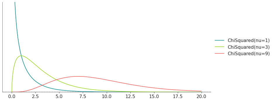
class preliz.distributions.chi_squared.ChiSquared(nu=None)[source]#

Chi squared distribution.

The pdf of this distribution is

\[f(x \mid \nu) = \frac{x^{(\nu-2)/2}e^{-x/2}}{2^{\nu/2}\Gamma(\nu/2)}\]

(Source code, png, hires.png, pdf)

Support	$x \in [0, \infty)$
Mean	$\nu$
Variance	$2 \nu$

Parameters:: nu (float) – Degrees of freedom (nu > 0).

cdf(x)[source]#

Cumulative distribution function.

Parameters:: x (array_like) – Values on which to evaluate the cdf

entropy()[source]#: Entropy.

eti(mass=None, fmt='.2f')#

Equal-tailed interval containing mass.

Parameters:

mass (float) – Probability mass in the interval. Defaults to None,
used. (which results in the value of rcParams["stats.ci_prob"] being)
fmt (str) – fmt used to represent results using f-string fmt for floats. Default to “.2f” i.e. 2 digits after the decimal point. Use “none” for no format.

hdi(mass=None, fmt='.2f')#

Highest density interval containing mass.

Parameters:

mass (float) – Probability mass in the interval. Defaults to None,
used. (which results in the value of rcParams["stats.ci_prob"] being)
fmt (str) – fmt used to represent results using f-string fmt for floats. Default to “.2f” i.e. 2 digits after the decimal point. Use “none” for no format.

isf(x)#

Inverse survival function (inverse of sf).

Parameters:: x (array_like) – Values on which to evaluate the inverse of the sf

kurtosis()[source]#: Excess kurtosis.

lmoment1()[source]#: L-moment1 (mean).

lmoment2()[source]#: L-moment2 (l-scale).

lmoment3()[source]#: L-moment3 (l-skewness). This the ratio of L-moment3 to L-moment2.

lmoment4()[source]#: L-moment4 (l-kurtosis). This the ratio of L-moment4 to L-moment2.

lmoments(types='1234')#

Compute L-moments of the distribution.

Parameters:: types (str) – The type of moments to compute. Default is ‘1234’ where ‘1’ = L-moment1 (mean), ‘2’ = L-moment2 (l-scale), ‘3’ = L-moment3 (l-skewness), and ‘4’ = L-moment4 (l-kurtosis). To compute the standard deviation use ‘d’ Valid combinations are any subset of ‘1234’.

logcdf(x)#

Log cumulative distribution function.

Parameters:: x (array_like) – Values on which to evaluate the logcdf

logpdf(x)[source]#

Log probability density/mass function.

Parameters:: x (array_like) – Values on which to evaluate the logpdf

logsf(x)#

Log survival function log(1 - cdf).

Parameters:: x (array_like) – Values on which to evaluate the logsf

mean()[source]#: Mean.

median()[source]#: Median.

mode()[source]#: Mode.

moments(types='mvsk')#

Compute moments of the distribution.

It can also return the standard deviation

Parameters:: types (str) – The type of moments to compute. Default is ‘mvsk’ where ‘m’ = mean, ‘v’ = variance, ‘s’ = skewness, and ‘k’ = kurtosis. To compute the standard deviation use ‘d’ Valid combinations are any subset of ‘mvdsk’.

pdf(x)[source]#

Probability density/mass function.

Parameters:: x (array_like) – Values on which to evaluate the pdf

plot_cdf(moments=None, pointinterval=False, interval=None, levels=None, support='restricted', legend='legend', figsize=None, ax=None, **kwargs)#

Plot the cumulative distribution function.

Parameters:

moments (str) – Compute moments. Use any combination of the strings m, d, v, s or k for the mean (μ), standard deviation (σ), variance (σ²), skew (γ) or kurtosis (κ) respectively. Other strings will be ignored. Defaults to None.
pointinterval (bool) – Whether to include a plot of the quantiles. Defaults to False. If True the default is to plot the median and two interquantiles ranges.
interval (str) – Type of interval. Available options are highest density interval “hdi” (default), equal tailed interval “eti” or intervals defined by arbitrary “quantiles”. Defaults to the value in rcParams[“stats.ci_kind”].
levels (list) – Mass of the intervals. For hdi or eti the number of elements should be 2 or 1. For quantiles the number of elements should be 5, 3, 1 or 0 (in this last case nothing will be plotted).
support (str:) – If full use the finite end-points to set the limits of the plot. For unbounded end-points or if restricted use the 0.001 and 0.999 quantiles to set the limits.
legend (str) – Whether to include a string with the distribution and its parameter as a "legend" a "title" or not include them None.
figsize (tuple) – Size of the figure
ax (matplotlib axes)
kwargs (keyword arguments) – Additional keyword arguments passed to matplotlib plot function. For example, color, alpha, linewidth, etc.

plot_interactive(kind='pdf', xy_lim='both', pointinterval=True, interval=None, levels=None, figsize=None)#

Interactive exploration of distributions parameters.

Parameters:

kind (str:) – Type of plot. Available options are pdf, cdf and ppf.
xy_lim (str or tuple) – Set the limits of the x-axis and/or y-axis. Defaults to “both”, the limits of both axis are fixed. Use “auto” for automatic rescaling of x-axis and y-axis. Or set them manually by passing a tuple of 4 elements, the first two for x-axis, the last two for y-axis. The tuple can have None.
pointinterval (bool) – Whether to include a plot of the quantiles. Defaults to False. If True the default is to plot the median and two interquantiles ranges.
interval (str) – Type of interval. Available options are highest density interval “hdi” (default), equal tailed interval “eti” or intervals defined by arbitrary “quantiles”. Defaults to the value in rcParams[“stats.ci_kind”].
levels (list) – Mass of the intervals. For hdi or eti the number of elements should be 2 or 1. For quantiles the number of elements should be 5, 3, 1 or 0 (in this last case nothing will be plotted).
figsize (tuple) – Size of the figure

plot_isf(moments=None, pointinterval=False, interval=None, levels=None, legend='legend', figsize=None, ax=None, **kwargs)#

Plot the inverse survival function.

Parameters:

moments (str) – Compute moments. Use any combination of the strings m, d, v, s or k for the mean (μ), standard deviation (σ), variance (σ²), skew (γ) or kurtosis (κ) respectively. Other strings will be ignored. Defaults to None.
pointinterval (bool) – Whether to include a plot of the quantiles. Defaults to False. If True the default is to plot the median and two interquantiles ranges.
interval (str) – Type of interval. Available options are highest density interval “hdi” (default), equal tailed interval “eti” or intervals defined by arbitrary “quantiles”. Defaults to the value in rcParams[“stats.ci_kind”].
levels (list) – Mass of the intervals. For hdi or eti the number of elements should be 2 or 1. For quantiles the number of elements should be 5, 3, 1 or 0 (in this last case nothing will be plotted).
legend (str) – Whether to include a string with the distribution and its parameter as a "legend" a "title" or not include them None.
figsize (tuple) – Size of the figure
ax (matplotlib axes)

plot_pdf(moments=None, pointinterval=False, interval=None, levels=None, support='restricted', baseline=True, legend='legend', figsize=None, ax=None, **kwargs)#

Plot the pdf (continuous) or pmf (discrete).

Parameters:

moments (str) – Compute moments. Use any combination of the strings m, d, v, s or k for the mean (μ), standard deviation (σ), variance (σ²), skew (γ) or kurtosis (κ) respectively. Other strings will be ignored. Defaults to None.
pointinterval (bool) – Whether to include a plot of the quantiles. Defaults to False. If True the default is to plot the median and two interquantiles ranges.
interval (str) – Type of interval. Available options are highest density interval “hdi” (default), equal tailed interval “eti” or intervals defined by arbitrary “quantiles”. Defaults to the value in rcParams[“stats.ci_kind”].
levels (list) – Mass of the intervals. For hdi or eti the number of elements should be 2 or 1. For quantiles the number of elements should be 5, 3, 1 or 0 (in this last case nothing will be plotted).
support (str:) – If full use the finite end-points to set the limits of the plot. For unbounded end-points or if restricted use the 0.001 and 0.999 quantiles to set the limits.
baseline (bool) – Whether to include a horizontal line at y=0.
legend (str) – Whether to include a string with the distribution and its parameter as a "legend" a "title" or not include them None.
figsize (tuple) – Size of the figure
ax (matplotlib axes)
kwargs (keyword arguments) – Additional keyword arguments passed to matplotlib plot function. For example, color, alpha, linewidth, etc.

plot_ppf(moments=None, pointinterval=False, interval=None, levels=None, legend='legend', figsize=None, ax=None, **kwargs)#

Plot the quantile function.

Parameters:

moments (str) – Compute moments. Use any combination of the strings m, d, v, s or k for the mean (μ), standard deviation (σ), variance (σ²), skew (γ) or kurtosis (κ) respectively. Other strings will be ignored. Defaults to None.
pointinterval (bool) – Whether to include a plot of the quantiles. Defaults to False. If True the default is to plot the median and two interquantiles ranges.
interval (str) – Type of interval. Available options are highest density interval “hdi” (default), equal tailed interval “eti” or intervals defined by arbitrary “quantiles”. Defaults to the value in rcParams[“stats.ci_kind”].
levels (list) – Mass of the intervals. For hdi or eti the number of elements should be 2 or 1. For quantiles the number of elements should be 5, 3, 1 or 0 (in this last case nothing will be plotted).
legend (str) – Whether to include a string with the distribution and its parameter as a "legend" a "title" or not include them None.
figsize (tuple) – Size of the figure
ax (matplotlib axes)

plot_sf(moments=None, pointinterval=False, interval=None, levels=None, support='restricted', legend='legend', figsize=None, ax=None, **kwargs)#

Plot the survival distribution function (1 - CDF).

Parameters:

moments (str) – Compute moments. Use any combination of the strings m, d, v, s or k for the mean (μ), standard deviation (σ), variance (σ²), skew (γ) or kurtosis (κ) respectively. Other strings will be ignored. Defaults to None.
pointinterval (bool) – Whether to include a plot of the quantiles. Defaults to False. If True the default is to plot the median and two interquantiles ranges.
interval (str) – Type of interval. Available options are highest density interval “hdi” (default), equal tailed interval “eti” or intervals defined by arbitrary “quantiles”. Defaults to the value in rcParams[“stats.ci_kind”].
levels (list) – Mass of the intervals. For hdi or eti the number of elements should be 2 or 1. For quantiles the number of elements should be 5, 3, 1 or 0 (in this last case nothing will be plotted).
support (str:) – If full use the finite end-points to set the limits of the plot. For unbounded end-points or if restricted use the 0.001 and 0.999 quantiles to set the limits.
legend (str) – Whether to include a string with the distribution and its parameter as a "legend" a "title" or not include them None.
figsize (tuple) – Size of the figure
ax (matplotlib axes)
kwargs (keyword arguments) – Additional keyword arguments passed to matplotlib plot function. For example, color, alpha, linewidth, etc.

ppf(q)[source]#

Percent point function (inverse of cdf).

Parameters:: x (array_like) – Values on which to evaluate the inverse of the cdf

rvs(size=None, random_state=None)[source]#

Random sample.

Parameters:

size (int or tuple of ints, optional) – Defining number of random variates. Defaults to 1.
random_state ({None, int, numpy.random.Generator, numpy.random.RandomState}) – Defaults to None

sf(x)#

Survival function (1 - cdf).

Parameters:: x (array_like) – Values on which to evaluate the sf

skewness()[source]#: Skewness.

std()[source]#: Standard deviation.

summary(mass=None, interval=None, fmt='.2f')#

Namedtuple with the mean, median, sd, and lower and upper bounds.

Parameters:

mass (float) – Probability mass for the equal-tailed interval. Defaults to None,
used. (which results in the value of rcParams["stats.ci_prob"] being)
interval (str or list-like) – Type of interval. Available options are highest density interval “hdi”, equal tailed interval “eti” or arbitrary interval defined by a list-like object with a pair of values. Defaults to the value in rcParams[“stats.ci_kind”].
fmt (str) – fmt used to represent results using f-string fmt for floats. Default to “.2f” i.e. 2 digits after the decimal point.

to_bambi(**kwargs)#

Convert the PreliZ distribution to a Bambi Prior.

kwargsPyMC distributions properties: kwargs are used to specify properties such as shape or dims

Return type:: Bambi Prior

to_pymc(name=None, **kwargs)#

Convert the PreliZ distribution to a PyMC distribution.

namestr: Name of PyMC distribution. Needed if inside Model context
kwargsPyMC distributions properties: kwargs are used to specify properties such as shape or dims

Return type:: PyMC distribution

var()[source]#: Variance.

xvals(support, n_points=None)#

Provide x values in the support of the distribution.

This is useful for example when plotting.

Parameters:

support (str) – Available options are “full” or “restricted”. If “full” the values will cover the entire support of the distribution if the boundary is finite, or the quantiles 0.0001 or 0.9999, if infinite. If “restricted” the values will cover the quantile 0.0001 to 0.9999.
n_points (int) – Number of values to return. Defaults to 1000 for continuous distributions and 200 for discrete ones. For discrete distributions the returned values may be fewer than n_points if the actual number of discrete values in the support of the distribution is smaller than n_points.

class preliz.distributions.exgaussian.ExGaussian(mu=None, sigma=None, nu=None)[source]#

Exponentially modified Gaussian (EMG) Distribution.

Results from the convolution of a normal distribution with an exponential distribution.

The pdf of this distribution is

\[f(x \mid \mu, \sigma, \nu) = \frac{1}{\nu}\; \exp\left\{\frac{\mu-x}{\nu}+\frac{\sigma^2}{2\nu^2}\right\} \Phi\left(\frac{x-\mu}{\sigma}-\frac{\sigma}{\nu}\right)\]

where $\Phi$ is the cumulative distribution function of the standard normal distribution.

(Source code, png, hires.png, pdf)

Support	$x \in \mathbb{R}$
Mean	$\mu + \nu$
Variance	$\sigma^2 + \nu^2$

Parameters:

mu (float) – Mean of the normal distribution.
sigma (float) – Standard deviation of the normal distribution (sigma > 0).
nu (float) – Mean of the exponential distribution (nu > 0).

cdf(x)[source]#

Cumulative distribution function.

Parameters:: x (array_like) – Values on which to evaluate the cdf

entropy()[source]#: Entropy.

eti(mass=None, fmt='.2f')#

Equal-tailed interval containing mass.

Parameters:

mass (float) – Probability mass in the interval. Defaults to None,
used. (which results in the value of rcParams["stats.ci_prob"] being)
fmt (str) – fmt used to represent results using f-string fmt for floats. Default to “.2f” i.e. 2 digits after the decimal point. Use “none” for no format.

hdi(mass=None, fmt='.2f')#

Highest density interval containing mass.

Parameters:

mass (float) – Probability mass in the interval. Defaults to None,
used. (which results in the value of rcParams["stats.ci_prob"] being)
fmt (str) – fmt used to represent results using f-string fmt for floats. Default to “.2f” i.e. 2 digits after the decimal point. Use “none” for no format.

isf(x)#

Inverse survival function (inverse of sf).

Parameters:: x (array_like) – Values on which to evaluate the inverse of the sf

kurtosis()[source]#: Excess kurtosis.

lmoment1()[source]#: L-moment1 (mean).

lmoment2()[source]#: L-moment2 (l-scale).

lmoment3()[source]#: L-moment3 (l-skewness). This the ratio of L-moment3 to L-moment2.

lmoment4()[source]#: L-moment4 (l-kurtosis). This the ratio of L-moment4 to L-moment2.

lmoments(types='1234')#

Compute L-moments of the distribution.

Parameters:: types (str) – The type of moments to compute. Default is ‘1234’ where ‘1’ = L-moment1 (mean), ‘2’ = L-moment2 (l-scale), ‘3’ = L-moment3 (l-skewness), and ‘4’ = L-moment4 (l-kurtosis). To compute the standard deviation use ‘d’ Valid combinations are any subset of ‘1234’.

logcdf(x)#

Log cumulative distribution function.

Parameters:: x (array_like) – Values on which to evaluate the logcdf

logpdf(x)[source]#

Log probability density/mass function.

Parameters:: x (array_like) – Values on which to evaluate the logpdf

logsf(x)#

Log survival function log(1 - cdf).

Parameters:: x (array_like) – Values on which to evaluate the logsf

mean()[source]#: Mean.

median()[source]#: Median.

mode()#: Mode.

moments(types='mvsk')#

Compute moments of the distribution.

It can also return the standard deviation

Parameters:: types (str) – The type of moments to compute. Default is ‘mvsk’ where ‘m’ = mean, ‘v’ = variance, ‘s’ = skewness, and ‘k’ = kurtosis. To compute the standard deviation use ‘d’ Valid combinations are any subset of ‘mvdsk’.

pdf(x)[source]#

Probability density/mass function.

Parameters:: x (array_like) – Values on which to evaluate the pdf

plot_cdf(moments=None, pointinterval=False, interval=None, levels=None, support='restricted', legend='legend', figsize=None, ax=None, **kwargs)#

Plot the cumulative distribution function.

Parameters:

moments (str) – Compute moments. Use any combination of the strings m, d, v, s or k for the mean (μ), standard deviation (σ), variance (σ²), skew (γ) or kurtosis (κ) respectively. Other strings will be ignored. Defaults to None.
pointinterval (bool) – Whether to include a plot of the quantiles. Defaults to False. If True the default is to plot the median and two interquantiles ranges.
interval (str) – Type of interval. Available options are highest density interval “hdi” (default), equal tailed interval “eti” or intervals defined by arbitrary “quantiles”. Defaults to the value in rcParams[“stats.ci_kind”].
levels (list) – Mass of the intervals. For hdi or eti the number of elements should be 2 or 1. For quantiles the number of elements should be 5, 3, 1 or 0 (in this last case nothing will be plotted).
support (str:) – If full use the finite end-points to set the limits of the plot. For unbounded end-points or if restricted use the 0.001 and 0.999 quantiles to set the limits.
legend (str) – Whether to include a string with the distribution and its parameter as a "legend" a "title" or not include them None.
figsize (tuple) – Size of the figure
ax (matplotlib axes)
kwargs (keyword arguments) – Additional keyword arguments passed to matplotlib plot function. For example, color, alpha, linewidth, etc.

plot_interactive(kind='pdf', xy_lim='both', pointinterval=True, interval=None, levels=None, figsize=None)#

Interactive exploration of distributions parameters.

Parameters:

kind (str:) – Type of plot. Available options are pdf, cdf and ppf.
xy_lim (str or tuple) – Set the limits of the x-axis and/or y-axis. Defaults to “both”, the limits of both axis are fixed. Use “auto” for automatic rescaling of x-axis and y-axis. Or set them manually by passing a tuple of 4 elements, the first two for x-axis, the last two for y-axis. The tuple can have None.
pointinterval (bool) – Whether to include a plot of the quantiles. Defaults to False. If True the default is to plot the median and two interquantiles ranges.
interval (str) – Type of interval. Available options are highest density interval “hdi” (default), equal tailed interval “eti” or intervals defined by arbitrary “quantiles”. Defaults to the value in rcParams[“stats.ci_kind”].
levels (list) – Mass of the intervals. For hdi or eti the number of elements should be 2 or 1. For quantiles the number of elements should be 5, 3, 1 or 0 (in this last case nothing will be plotted).
figsize (tuple) – Size of the figure

plot_isf(moments=None, pointinterval=False, interval=None, levels=None, legend='legend', figsize=None, ax=None, **kwargs)#

Plot the inverse survival function.

Parameters:

moments (str) – Compute moments. Use any combination of the strings m, d, v, s or k for the mean (μ), standard deviation (σ), variance (σ²), skew (γ) or kurtosis (κ) respectively. Other strings will be ignored. Defaults to None.
pointinterval (bool) – Whether to include a plot of the quantiles. Defaults to False. If True the default is to plot the median and two interquantiles ranges.
interval (str) – Type of interval. Available options are highest density interval “hdi” (default), equal tailed interval “eti” or intervals defined by arbitrary “quantiles”. Defaults to the value in rcParams[“stats.ci_kind”].
levels (list) – Mass of the intervals. For hdi or eti the number of elements should be 2 or 1. For quantiles the number of elements should be 5, 3, 1 or 0 (in this last case nothing will be plotted).
legend (str) – Whether to include a string with the distribution and its parameter as a "legend" a "title" or not include them None.
figsize (tuple) – Size of the figure
ax (matplotlib axes)

plot_pdf(moments=None, pointinterval=False, interval=None, levels=None, support='restricted', baseline=True, legend='legend', figsize=None, ax=None, **kwargs)#

Plot the pdf (continuous) or pmf (discrete).

Parameters:

moments (str) – Compute moments. Use any combination of the strings m, d, v, s or k for the mean (μ), standard deviation (σ), variance (σ²), skew (γ) or kurtosis (κ) respectively. Other strings will be ignored. Defaults to None.
pointinterval (bool) – Whether to include a plot of the quantiles. Defaults to False. If True the default is to plot the median and two interquantiles ranges.
interval (str) – Type of interval. Available options are highest density interval “hdi” (default), equal tailed interval “eti” or intervals defined by arbitrary “quantiles”. Defaults to the value in rcParams[“stats.ci_kind”].
levels (list) – Mass of the intervals. For hdi or eti the number of elements should be 2 or 1. For quantiles the number of elements should be 5, 3, 1 or 0 (in this last case nothing will be plotted).
support (str:) – If full use the finite end-points to set the limits of the plot. For unbounded end-points or if restricted use the 0.001 and 0.999 quantiles to set the limits.
baseline (bool) – Whether to include a horizontal line at y=0.
legend (str) – Whether to include a string with the distribution and its parameter as a "legend" a "title" or not include them None.
figsize (tuple) – Size of the figure
ax (matplotlib axes)
kwargs (keyword arguments) – Additional keyword arguments passed to matplotlib plot function. For example, color, alpha, linewidth, etc.

plot_ppf(moments=None, pointinterval=False, interval=None, levels=None, legend='legend', figsize=None, ax=None, **kwargs)#

Plot the quantile function.

Parameters:

moments (str) – Compute moments. Use any combination of the strings m, d, v, s or k for the mean (μ), standard deviation (σ), variance (σ²), skew (γ) or kurtosis (κ) respectively. Other strings will be ignored. Defaults to None.
pointinterval (bool) – Whether to include a plot of the quantiles. Defaults to False. If True the default is to plot the median and two interquantiles ranges.
interval (str) – Type of interval. Available options are highest density interval “hdi” (default), equal tailed interval “eti” or intervals defined by arbitrary “quantiles”. Defaults to the value in rcParams[“stats.ci_kind”].
levels (list) – Mass of the intervals. For hdi or eti the number of elements should be 2 or 1. For quantiles the number of elements should be 5, 3, 1 or 0 (in this last case nothing will be plotted).
legend (str) – Whether to include a string with the distribution and its parameter as a "legend" a "title" or not include them None.
figsize (tuple) – Size of the figure
ax (matplotlib axes)

plot_sf(moments=None, pointinterval=False, interval=None, levels=None, support='restricted', legend='legend', figsize=None, ax=None, **kwargs)#

Plot the survival distribution function (1 - CDF).

Parameters:

moments (str) – Compute moments. Use any combination of the strings m, d, v, s or k for the mean (μ), standard deviation (σ), variance (σ²), skew (γ) or kurtosis (κ) respectively. Other strings will be ignored. Defaults to None.
pointinterval (bool) – Whether to include a plot of the quantiles. Defaults to False. If True the default is to plot the median and two interquantiles ranges.
interval (str) – Type of interval. Available options are highest density interval “hdi” (default), equal tailed interval “eti” or intervals defined by arbitrary “quantiles”. Defaults to the value in rcParams[“stats.ci_kind”].
levels (list) – Mass of the intervals. For hdi or eti the number of elements should be 2 or 1. For quantiles the number of elements should be 5, 3, 1 or 0 (in this last case nothing will be plotted).
support (str:) – If full use the finite end-points to set the limits of the plot. For unbounded end-points or if restricted use the 0.001 and 0.999 quantiles to set the limits.
legend (str) – Whether to include a string with the distribution and its parameter as a "legend" a "title" or not include them None.
figsize (tuple) – Size of the figure
ax (matplotlib axes)
kwargs (keyword arguments) – Additional keyword arguments passed to matplotlib plot function. For example, color, alpha, linewidth, etc.

ppf(q)[source]#

Percent point function (inverse of cdf).

Parameters:: x (array_like) – Values on which to evaluate the inverse of the cdf

rvs(size=None, random_state=None)[source]#

Random sample.

Parameters:

size (int or tuple of ints, optional) – Defining number of random variates. Defaults to 1.
random_state ({None, int, numpy.random.Generator, numpy.random.RandomState}) – Defaults to None

sf(x)#

Survival function (1 - cdf).

Parameters:: x (array_like) – Values on which to evaluate the sf

skewness()[source]#: Skewness.

std()[source]#: Standard deviation.

summary(mass=None, interval=None, fmt='.2f')#

Namedtuple with the mean, median, sd, and lower and upper bounds.

Parameters:

mass (float) – Probability mass for the equal-tailed interval. Defaults to None,
used. (which results in the value of rcParams["stats.ci_prob"] being)
interval (str or list-like) – Type of interval. Available options are highest density interval “hdi”, equal tailed interval “eti” or arbitrary interval defined by a list-like object with a pair of values. Defaults to the value in rcParams[“stats.ci_kind”].
fmt (str) – fmt used to represent results using f-string fmt for floats. Default to “.2f” i.e. 2 digits after the decimal point.

to_bambi(**kwargs)#

Convert the PreliZ distribution to a Bambi Prior.

kwargsPyMC distributions properties: kwargs are used to specify properties such as shape or dims

Return type:: Bambi Prior

to_pymc(name=None, **kwargs)#

Convert the PreliZ distribution to a PyMC distribution.

namestr: Name of PyMC distribution. Needed if inside Model context
kwargsPyMC distributions properties: kwargs are used to specify properties such as shape or dims

Return type:: PyMC distribution

var()[source]#: Variance.

xvals(support, n_points=None)#

Provide x values in the support of the distribution.

This is useful for example when plotting.

Parameters:

support (str) – Available options are “full” or “restricted”. If “full” the values will cover the entire support of the distribution if the boundary is finite, or the quantiles 0.0001 or 0.9999, if infinite. If “restricted” the values will cover the quantile 0.0001 to 0.9999.
n_points (int) – Number of values to return. Defaults to 1000 for continuous distributions and 200 for discrete ones. For discrete distributions the returned values may be fewer than n_points if the actual number of discrete values in the support of the distribution is smaller than n_points.

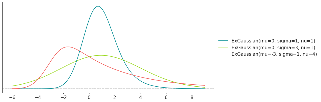
class preliz.distributions.exponential.Exponential(lam=None, scale=None)[source]#

Exponential Distribution.

The pdf of this distribution is

\[f(x \mid \lambda) = \lambda \exp\left\{ -\lambda x \right\}\]

(Source code, png, hires.png, pdf)

Support	$x \in [0, \infty)$
Mean	$\dfrac{1}{\lambda}$
Variance	$\dfrac{1}{\lambda^2}$

Exponential distribution has 2 alternative parametrizations. In terms of lambda (rate) or in terms of scale.

The link between the two alternatives is given by:

\[scale = \dfrac{1}{\lambda}\]

Parameters:

lam (float) – Rate or inverse scale (lam > 0).
scale (float) – Scale (scale > 0).

cdf(x)[source]#

Cumulative distribution function.

Parameters:: x (array_like) – Values on which to evaluate the cdf

entropy()[source]#: Entropy.

eti(mass=None, fmt='.2f')#

Equal-tailed interval containing mass.

Parameters:

mass (float) – Probability mass in the interval. Defaults to None,
used. (which results in the value of rcParams["stats.ci_prob"] being)
fmt (str) – fmt used to represent results using f-string fmt for floats. Default to “.2f” i.e. 2 digits after the decimal point. Use “none” for no format.

hdi(mass=None, fmt='.2f')#

Highest density interval containing mass.

Parameters:

mass (float) – Probability mass in the interval. Defaults to None,
used. (which results in the value of rcParams["stats.ci_prob"] being)
fmt (str) – fmt used to represent results using f-string fmt for floats. Default to “.2f” i.e. 2 digits after the decimal point. Use “none” for no format.

isf(x)#

Inverse survival function (inverse of sf).

Parameters:: x (array_like) – Values on which to evaluate the inverse of the sf

kurtosis()[source]#: Excess kurtosis.

lmoment1()[source]#: L-moment1 (mean).

lmoment2()[source]#: L-moment2 (l-scale).

lmoment3()[source]#: L-moment3 (l-skewness). This the ratio of L-moment3 to L-moment2.

lmoment4()[source]#: L-moment4 (l-kurtosis). This the ratio of L-moment4 to L-moment2.

lmoments(types='1234')#

Compute L-moments of the distribution.

Parameters:: types (str) – The type of moments to compute. Default is ‘1234’ where ‘1’ = L-moment1 (mean), ‘2’ = L-moment2 (l-scale), ‘3’ = L-moment3 (l-skewness), and ‘4’ = L-moment4 (l-kurtosis). To compute the standard deviation use ‘d’ Valid combinations are any subset of ‘1234’.

logcdf(x)#

Log cumulative distribution function.

Parameters:: x (array_like) – Values on which to evaluate the logcdf

logpdf(x)[source]#

Log probability density/mass function.

Parameters:: x (array_like) – Values on which to evaluate the logpdf

logsf(x)#

Log survival function log(1 - cdf).

Parameters:: x (array_like) – Values on which to evaluate the logsf

mean()[source]#: Mean.

median()[source]#: Median.

mode()[source]#: Mode.

moments(types='mvsk')#

Compute moments of the distribution.

It can also return the standard deviation

Parameters:: types (str) – The type of moments to compute. Default is ‘mvsk’ where ‘m’ = mean, ‘v’ = variance, ‘s’ = skewness, and ‘k’ = kurtosis. To compute the standard deviation use ‘d’ Valid combinations are any subset of ‘mvdsk’.

pdf(x)[source]#

Probability density/mass function.

Parameters:: x (array_like) – Values on which to evaluate the pdf

plot_cdf(moments=None, pointinterval=False, interval=None, levels=None, support='restricted', legend='legend', figsize=None, ax=None, **kwargs)#

Plot the cumulative distribution function.

Parameters:

moments (str) – Compute moments. Use any combination of the strings m, d, v, s or k for the mean (μ), standard deviation (σ), variance (σ²), skew (γ) or kurtosis (κ) respectively. Other strings will be ignored. Defaults to None.
pointinterval (bool) – Whether to include a plot of the quantiles. Defaults to False. If True the default is to plot the median and two interquantiles ranges.
interval (str) – Type of interval. Available options are highest density interval “hdi” (default), equal tailed interval “eti” or intervals defined by arbitrary “quantiles”. Defaults to the value in rcParams[“stats.ci_kind”].
levels (list) – Mass of the intervals. For hdi or eti the number of elements should be 2 or 1. For quantiles the number of elements should be 5, 3, 1 or 0 (in this last case nothing will be plotted).
support (str:) – If full use the finite end-points to set the limits of the plot. For unbounded end-points or if restricted use the 0.001 and 0.999 quantiles to set the limits.
legend (str) – Whether to include a string with the distribution and its parameter as a "legend" a "title" or not include them None.
figsize (tuple) – Size of the figure
ax (matplotlib axes)
kwargs (keyword arguments) – Additional keyword arguments passed to matplotlib plot function. For example, color, alpha, linewidth, etc.

plot_interactive(kind='pdf', xy_lim='both', pointinterval=True, interval=None, levels=None, figsize=None)#

Interactive exploration of distributions parameters.

Parameters:

kind (str:) – Type of plot. Available options are pdf, cdf and ppf.
xy_lim (str or tuple) – Set the limits of the x-axis and/or y-axis. Defaults to “both”, the limits of both axis are fixed. Use “auto” for automatic rescaling of x-axis and y-axis. Or set them manually by passing a tuple of 4 elements, the first two for x-axis, the last two for y-axis. The tuple can have None.
pointinterval (bool) – Whether to include a plot of the quantiles. Defaults to False. If True the default is to plot the median and two interquantiles ranges.
interval (str) – Type of interval. Available options are highest density interval “hdi” (default), equal tailed interval “eti” or intervals defined by arbitrary “quantiles”. Defaults to the value in rcParams[“stats.ci_kind”].
levels (list) – Mass of the intervals. For hdi or eti the number of elements should be 2 or 1. For quantiles the number of elements should be 5, 3, 1 or 0 (in this last case nothing will be plotted).
figsize (tuple) – Size of the figure

plot_isf(moments=None, pointinterval=False, interval=None, levels=None, legend='legend', figsize=None, ax=None, **kwargs)#

Plot the inverse survival function.

Parameters:

moments (str) – Compute moments. Use any combination of the strings m, d, v, s or k for the mean (μ), standard deviation (σ), variance (σ²), skew (γ) or kurtosis (κ) respectively. Other strings will be ignored. Defaults to None.
pointinterval (bool) – Whether to include a plot of the quantiles. Defaults to False. If True the default is to plot the median and two interquantiles ranges.
interval (str) – Type of interval. Available options are highest density interval “hdi” (default), equal tailed interval “eti” or intervals defined by arbitrary “quantiles”. Defaults to the value in rcParams[“stats.ci_kind”].
levels (list) – Mass of the intervals. For hdi or eti the number of elements should be 2 or 1. For quantiles the number of elements should be 5, 3, 1 or 0 (in this last case nothing will be plotted).
legend (str) – Whether to include a string with the distribution and its parameter as a "legend" a "title" or not include them None.
figsize (tuple) – Size of the figure
ax (matplotlib axes)

plot_pdf(moments=None, pointinterval=False, interval=None, levels=None, support='restricted', baseline=True, legend='legend', figsize=None, ax=None, **kwargs)#

Plot the pdf (continuous) or pmf (discrete).

Parameters:

moments (str) – Compute moments. Use any combination of the strings m, d, v, s or k for the mean (μ), standard deviation (σ), variance (σ²), skew (γ) or kurtosis (κ) respectively. Other strings will be ignored. Defaults to None.
pointinterval (bool) – Whether to include a plot of the quantiles. Defaults to False. If True the default is to plot the median and two interquantiles ranges.
interval (str) – Type of interval. Available options are highest density interval “hdi” (default), equal tailed interval “eti” or intervals defined by arbitrary “quantiles”. Defaults to the value in rcParams[“stats.ci_kind”].
levels (list) – Mass of the intervals. For hdi or eti the number of elements should be 2 or 1. For quantiles the number of elements should be 5, 3, 1 or 0 (in this last case nothing will be plotted).
support (str:) – If full use the finite end-points to set the limits of the plot. For unbounded end-points or if restricted use the 0.001 and 0.999 quantiles to set the limits.
baseline (bool) – Whether to include a horizontal line at y=0.
legend (str) – Whether to include a string with the distribution and its parameter as a "legend" a "title" or not include them None.
figsize (tuple) – Size of the figure
ax (matplotlib axes)
kwargs (keyword arguments) – Additional keyword arguments passed to matplotlib plot function. For example, color, alpha, linewidth, etc.

plot_ppf(moments=None, pointinterval=False, interval=None, levels=None, legend='legend', figsize=None, ax=None, **kwargs)#

Plot the quantile function.

Parameters:

moments (str) – Compute moments. Use any combination of the strings m, d, v, s or k for the mean (μ), standard deviation (σ), variance (σ²), skew (γ) or kurtosis (κ) respectively. Other strings will be ignored. Defaults to None.
pointinterval (bool) – Whether to include a plot of the quantiles. Defaults to False. If True the default is to plot the median and two interquantiles ranges.
interval (str) – Type of interval. Available options are highest density interval “hdi” (default), equal tailed interval “eti” or intervals defined by arbitrary “quantiles”. Defaults to the value in rcParams[“stats.ci_kind”].
levels (list) – Mass of the intervals. For hdi or eti the number of elements should be 2 or 1. For quantiles the number of elements should be 5, 3, 1 or 0 (in this last case nothing will be plotted).
legend (str) – Whether to include a string with the distribution and its parameter as a "legend" a "title" or not include them None.
figsize (tuple) – Size of the figure
ax (matplotlib axes)

plot_sf(moments=None, pointinterval=False, interval=None, levels=None, support='restricted', legend='legend', figsize=None, ax=None, **kwargs)#

Plot the survival distribution function (1 - CDF).

Parameters:

moments (str) – Compute moments. Use any combination of the strings m, d, v, s or k for the mean (μ), standard deviation (σ), variance (σ²), skew (γ) or kurtosis (κ) respectively. Other strings will be ignored. Defaults to None.
pointinterval (bool) – Whether to include a plot of the quantiles. Defaults to False. If True the default is to plot the median and two interquantiles ranges.
interval (str) – Type of interval. Available options are highest density interval “hdi” (default), equal tailed interval “eti” or intervals defined by arbitrary “quantiles”. Defaults to the value in rcParams[“stats.ci_kind”].
levels (list) – Mass of the intervals. For hdi or eti the number of elements should be 2 or 1. For quantiles the number of elements should be 5, 3, 1 or 0 (in this last case nothing will be plotted).
support (str:) – If full use the finite end-points to set the limits of the plot. For unbounded end-points or if restricted use the 0.001 and 0.999 quantiles to set the limits.
legend (str) – Whether to include a string with the distribution and its parameter as a "legend" a "title" or not include them None.
figsize (tuple) – Size of the figure
ax (matplotlib axes)
kwargs (keyword arguments) – Additional keyword arguments passed to matplotlib plot function. For example, color, alpha, linewidth, etc.

ppf(q)[source]#

Percent point function (inverse of cdf).

Parameters:: x (array_like) – Values on which to evaluate the inverse of the cdf

rvs(size=None, random_state=None)[source]#

Random sample.

Parameters:

size (int or tuple of ints, optional) – Defining number of random variates. Defaults to 1.
random_state ({None, int, numpy.random.Generator, numpy.random.RandomState}) – Defaults to None

sf(x)#

Survival function (1 - cdf).

Parameters:: x (array_like) – Values on which to evaluate the sf

skewness()[source]#: Skewness.

std()[source]#: Standard deviation.

summary(mass=None, interval=None, fmt='.2f')#

Namedtuple with the mean, median, sd, and lower and upper bounds.

Parameters:

mass (float) – Probability mass for the equal-tailed interval. Defaults to None,
used. (which results in the value of rcParams["stats.ci_prob"] being)
interval (str or list-like) – Type of interval. Available options are highest density interval “hdi”, equal tailed interval “eti” or arbitrary interval defined by a list-like object with a pair of values. Defaults to the value in rcParams[“stats.ci_kind”].
fmt (str) – fmt used to represent results using f-string fmt for floats. Default to “.2f” i.e. 2 digits after the decimal point.

to_bambi(**kwargs)#

Convert the PreliZ distribution to a Bambi Prior.

kwargsPyMC distributions properties: kwargs are used to specify properties such as shape or dims

Return type:: Bambi Prior

to_pymc(name=None, **kwargs)#

Convert the PreliZ distribution to a PyMC distribution.

namestr: Name of PyMC distribution. Needed if inside Model context
kwargsPyMC distributions properties: kwargs are used to specify properties such as shape or dims

Return type:: PyMC distribution

var()[source]#: Variance.

xvals(support, n_points=None)#

Provide x values in the support of the distribution.

This is useful for example when plotting.

Parameters:

support (str) – Available options are “full” or “restricted”. If “full” the values will cover the entire support of the distribution if the boundary is finite, or the quantiles 0.0001 or 0.9999, if infinite. If “restricted” the values will cover the quantile 0.0001 to 0.9999.
n_points (int) – Number of values to return. Defaults to 1000 for continuous distributions and 200 for discrete ones. For discrete distributions the returned values may be fewer than n_points if the actual number of discrete values in the support of the distribution is smaller than n_points.

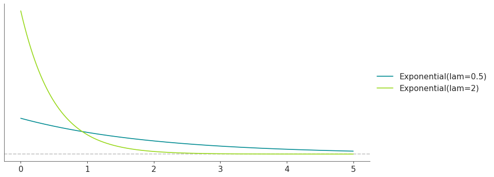
class preliz.distributions.gamma.Gamma(alpha=None, beta=None, mu=None, sigma=None)[source]#

Gamma distribution.

Represents the sum of alpha exponentially distributed random variables, each of which has rate beta.

The pdf of this distribution is

\[f(x \mid \alpha, \beta) = \frac{\beta^{\alpha}x^{\alpha-1}e^{-\beta x}}{\Gamma(\alpha)}\]

(Source code, png, hires.png, pdf)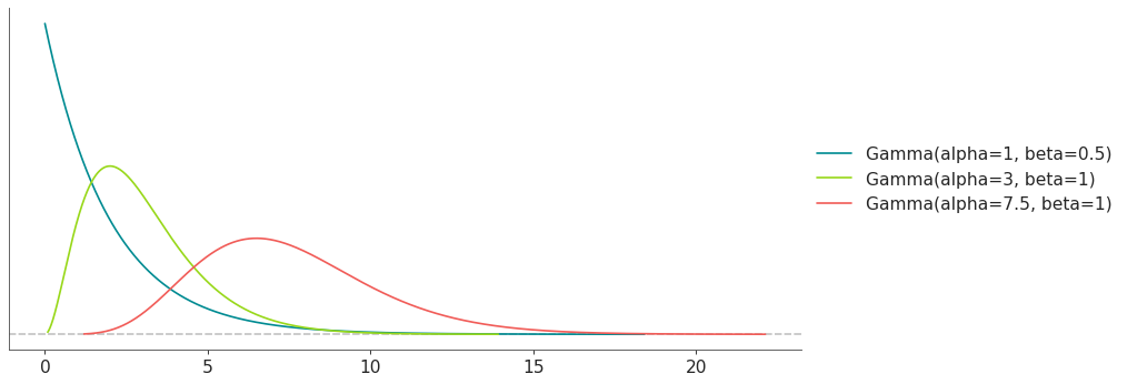

Support	$x \in (0, \infty)$
Mean	$\dfrac{\alpha}{\beta}$
Variance	$\dfrac{\alpha}{\beta^2}$

Gamma distribution has 2 alternative parameterizations. In terms of alpha and beta or mu (mean) and sigma (standard deviation).

The link between the 2 alternatives is given by

\[\begin{split}\alpha &= \frac{\mu^2}{\sigma^2} \\ \beta &= \frac{\mu}{\sigma^2}\end{split}\]

Parameters:

alpha (float) – Shape parameter (alpha > 0).
beta (float) – Rate parameter (beta > 0).
mu (float) – Mean (mu > 0).
sigma (float) – Standard deviation (sigma > 0)

cdf(x)[source]#

Cumulative distribution function.

Parameters:: x (array_like) – Values on which to evaluate the cdf

entropy()[source]#: Entropy.

eti(mass=None, fmt='.2f')#

Equal-tailed interval containing mass.

Parameters:

mass (float) – Probability mass in the interval. Defaults to None,
used. (which results in the value of rcParams["stats.ci_prob"] being)
fmt (str) – fmt used to represent results using f-string fmt for floats. Default to “.2f” i.e. 2 digits after the decimal point. Use “none” for no format.

hdi(mass=None, fmt='.2f')#

Highest density interval containing mass.

Parameters:

mass (float) – Probability mass in the interval. Defaults to None,
used. (which results in the value of rcParams["stats.ci_prob"] being)
fmt (str) – fmt used to represent results using f-string fmt for floats. Default to “.2f” i.e. 2 digits after the decimal point. Use “none” for no format.

isf(x)#

Inverse survival function (inverse of sf).

Parameters:: x (array_like) – Values on which to evaluate the inverse of the sf

kurtosis()[source]#: Excess kurtosis.

lmoment1()[source]#: L-moment1 (mean).

lmoment2()[source]#: L-moment2 (l-scale).

lmoment3()[source]#: L-moment3 (l-skewness). This the ratio of L-moment3 to L-moment2.

lmoment4()[source]#: L-moment4 (l-kurtosis). This the ratio of L-moment4 to L-moment2.

lmoments(types='1234')#

Compute L-moments of the distribution.

Parameters:: types (str) – The type of moments to compute. Default is ‘1234’ where ‘1’ = L-moment1 (mean), ‘2’ = L-moment2 (l-scale), ‘3’ = L-moment3 (l-skewness), and ‘4’ = L-moment4 (l-kurtosis). To compute the standard deviation use ‘d’ Valid combinations are any subset of ‘1234’.

logcdf(x)#

Log cumulative distribution function.

Parameters:: x (array_like) – Values on which to evaluate the logcdf

logpdf(x)[source]#

Log probability density/mass function.

Parameters:: x (array_like) – Values on which to evaluate the logpdf

logsf(x)#

Log survival function log(1 - cdf).

Parameters:: x (array_like) – Values on which to evaluate the logsf

mean()[source]#: Mean.

median()[source]#: Median.

mode()[source]#: Mode.

moments(types='mvsk')#

Compute moments of the distribution.

It can also return the standard deviation

Parameters:: types (str) – The type of moments to compute. Default is ‘mvsk’ where ‘m’ = mean, ‘v’ = variance, ‘s’ = skewness, and ‘k’ = kurtosis. To compute the standard deviation use ‘d’ Valid combinations are any subset of ‘mvdsk’.

pdf(x)[source]#

Probability density/mass function.

Parameters:: x (array_like) – Values on which to evaluate the pdf

plot_cdf(moments=None, pointinterval=False, interval=None, levels=None, support='restricted', legend='legend', figsize=None, ax=None, **kwargs)#

Plot the cumulative distribution function.

Parameters:

moments (str) – Compute moments. Use any combination of the strings m, d, v, s or k for the mean (μ), standard deviation (σ), variance (σ²), skew (γ) or kurtosis (κ) respectively. Other strings will be ignored. Defaults to None.
pointinterval (bool) – Whether to include a plot of the quantiles. Defaults to False. If True the default is to plot the median and two interquantiles ranges.
interval (str) – Type of interval. Available options are highest density interval “hdi” (default), equal tailed interval “eti” or intervals defined by arbitrary “quantiles”. Defaults to the value in rcParams[“stats.ci_kind”].
levels (list) – Mass of the intervals. For hdi or eti the number of elements should be 2 or 1. For quantiles the number of elements should be 5, 3, 1 or 0 (in this last case nothing will be plotted).
support (str:) – If full use the finite end-points to set the limits of the plot. For unbounded end-points or if restricted use the 0.001 and 0.999 quantiles to set the limits.
legend (str) – Whether to include a string with the distribution and its parameter as a "legend" a "title" or not include them None.
figsize (tuple) – Size of the figure
ax (matplotlib axes)
kwargs (keyword arguments) – Additional keyword arguments passed to matplotlib plot function. For example, color, alpha, linewidth, etc.

plot_interactive(kind='pdf', xy_lim='both', pointinterval=True, interval=None, levels=None, figsize=None)#

Interactive exploration of distributions parameters.

Parameters:

kind (str:) – Type of plot. Available options are pdf, cdf and ppf.
xy_lim (str or tuple) – Set the limits of the x-axis and/or y-axis. Defaults to “both”, the limits of both axis are fixed. Use “auto” for automatic rescaling of x-axis and y-axis. Or set them manually by passing a tuple of 4 elements, the first two for x-axis, the last two for y-axis. The tuple can have None.
pointinterval (bool) – Whether to include a plot of the quantiles. Defaults to False. If True the default is to plot the median and two interquantiles ranges.
interval (str) – Type of interval. Available options are highest density interval “hdi” (default), equal tailed interval “eti” or intervals defined by arbitrary “quantiles”. Defaults to the value in rcParams[“stats.ci_kind”].
levels (list) – Mass of the intervals. For hdi or eti the number of elements should be 2 or 1. For quantiles the number of elements should be 5, 3, 1 or 0 (in this last case nothing will be plotted).
figsize (tuple) – Size of the figure

plot_isf(moments=None, pointinterval=False, interval=None, levels=None, legend='legend', figsize=None, ax=None, **kwargs)#

Plot the inverse survival function.

Parameters:

moments (str) – Compute moments. Use any combination of the strings m, d, v, s or k for the mean (μ), standard deviation (σ), variance (σ²), skew (γ) or kurtosis (κ) respectively. Other strings will be ignored. Defaults to None.
pointinterval (bool) – Whether to include a plot of the quantiles. Defaults to False. If True the default is to plot the median and two interquantiles ranges.
interval (str) – Type of interval. Available options are highest density interval “hdi” (default), equal tailed interval “eti” or intervals defined by arbitrary “quantiles”. Defaults to the value in rcParams[“stats.ci_kind”].
levels (list) – Mass of the intervals. For hdi or eti the number of elements should be 2 or 1. For quantiles the number of elements should be 5, 3, 1 or 0 (in this last case nothing will be plotted).
legend (str) – Whether to include a string with the distribution and its parameter as a "legend" a "title" or not include them None.
figsize (tuple) – Size of the figure
ax (matplotlib axes)

plot_pdf(moments=None, pointinterval=False, interval=None, levels=None, support='restricted', baseline=True, legend='legend', figsize=None, ax=None, **kwargs)#

Plot the pdf (continuous) or pmf (discrete).

Parameters:

moments (str) – Compute moments. Use any combination of the strings m, d, v, s or k for the mean (μ), standard deviation (σ), variance (σ²), skew (γ) or kurtosis (κ) respectively. Other strings will be ignored. Defaults to None.
pointinterval (bool) – Whether to include a plot of the quantiles. Defaults to False. If True the default is to plot the median and two interquantiles ranges.
interval (str) – Type of interval. Available options are highest density interval “hdi” (default), equal tailed interval “eti” or intervals defined by arbitrary “quantiles”. Defaults to the value in rcParams[“stats.ci_kind”].
levels (list) – Mass of the intervals. For hdi or eti the number of elements should be 2 or 1. For quantiles the number of elements should be 5, 3, 1 or 0 (in this last case nothing will be plotted).
support (str:) – If full use the finite end-points to set the limits of the plot. For unbounded end-points or if restricted use the 0.001 and 0.999 quantiles to set the limits.
baseline (bool) – Whether to include a horizontal line at y=0.
legend (str) – Whether to include a string with the distribution and its parameter as a "legend" a "title" or not include them None.
figsize (tuple) – Size of the figure
ax (matplotlib axes)
kwargs (keyword arguments) – Additional keyword arguments passed to matplotlib plot function. For example, color, alpha, linewidth, etc.

plot_ppf(moments=None, pointinterval=False, interval=None, levels=None, legend='legend', figsize=None, ax=None, **kwargs)#

Plot the quantile function.

Parameters:

moments (str) – Compute moments. Use any combination of the strings m, d, v, s or k for the mean (μ), standard deviation (σ), variance (σ²), skew (γ) or kurtosis (κ) respectively. Other strings will be ignored. Defaults to None.
pointinterval (bool) – Whether to include a plot of the quantiles. Defaults to False. If True the default is to plot the median and two interquantiles ranges.
interval (str) – Type of interval. Available options are highest density interval “hdi” (default), equal tailed interval “eti” or intervals defined by arbitrary “quantiles”. Defaults to the value in rcParams[“stats.ci_kind”].
levels (list) – Mass of the intervals. For hdi or eti the number of elements should be 2 or 1. For quantiles the number of elements should be 5, 3, 1 or 0 (in this last case nothing will be plotted).
legend (str) – Whether to include a string with the distribution and its parameter as a "legend" a "title" or not include them None.
figsize (tuple) – Size of the figure
ax (matplotlib axes)

plot_sf(moments=None, pointinterval=False, interval=None, levels=None, support='restricted', legend='legend', figsize=None, ax=None, **kwargs)#

Plot the survival distribution function (1 - CDF).

Parameters:

moments (str) – Compute moments. Use any combination of the strings m, d, v, s or k for the mean (μ), standard deviation (σ), variance (σ²), skew (γ) or kurtosis (κ) respectively. Other strings will be ignored. Defaults to None.
pointinterval (bool) – Whether to include a plot of the quantiles. Defaults to False. If True the default is to plot the median and two interquantiles ranges.
interval (str) – Type of interval. Available options are highest density interval “hdi” (default), equal tailed interval “eti” or intervals defined by arbitrary “quantiles”. Defaults to the value in rcParams[“stats.ci_kind”].
levels (list) – Mass of the intervals. For hdi or eti the number of elements should be 2 or 1. For quantiles the number of elements should be 5, 3, 1 or 0 (in this last case nothing will be plotted).
support (str:) – If full use the finite end-points to set the limits of the plot. For unbounded end-points or if restricted use the 0.001 and 0.999 quantiles to set the limits.
legend (str) – Whether to include a string with the distribution and its parameter as a "legend" a "title" or not include them None.
figsize (tuple) – Size of the figure
ax (matplotlib axes)
kwargs (keyword arguments) – Additional keyword arguments passed to matplotlib plot function. For example, color, alpha, linewidth, etc.

ppf(q)[source]#

Percent point function (inverse of cdf).

Parameters:: x (array_like) – Values on which to evaluate the inverse of the cdf

rvs(size=None, random_state=None)[source]#

Random sample.

Parameters:

size (int or tuple of ints, optional) – Defining number of random variates. Defaults to 1.
random_state ({None, int, numpy.random.Generator, numpy.random.RandomState}) – Defaults to None

sf(x)#

Survival function (1 - cdf).

Parameters:: x (array_like) – Values on which to evaluate the sf

skewness()[source]#: Skewness.

std()[source]#: Standard deviation.

summary(mass=None, interval=None, fmt='.2f')#

Namedtuple with the mean, median, sd, and lower and upper bounds.

Parameters:

mass (float) – Probability mass for the equal-tailed interval. Defaults to None,
used. (which results in the value of rcParams["stats.ci_prob"] being)
interval (str or list-like) – Type of interval. Available options are highest density interval “hdi”, equal tailed interval “eti” or arbitrary interval defined by a list-like object with a pair of values. Defaults to the value in rcParams[“stats.ci_kind”].
fmt (str) – fmt used to represent results using f-string fmt for floats. Default to “.2f” i.e. 2 digits after the decimal point.

to_bambi(**kwargs)#

Convert the PreliZ distribution to a Bambi Prior.

kwargsPyMC distributions properties: kwargs are used to specify properties such as shape or dims

Return type:: Bambi Prior

to_pymc(name=None, **kwargs)#

Convert the PreliZ distribution to a PyMC distribution.

namestr: Name of PyMC distribution. Needed if inside Model context
kwargsPyMC distributions properties: kwargs are used to specify properties such as shape or dims

Return type:: PyMC distribution

var()[source]#: Variance.

xvals(support, n_points=None)#

Provide x values in the support of the distribution.

This is useful for example when plotting.

Parameters:

support (str) – Available options are “full” or “restricted”. If “full” the values will cover the entire support of the distribution if the boundary is finite, or the quantiles 0.0001 or 0.9999, if infinite. If “restricted” the values will cover the quantile 0.0001 to 0.9999.
n_points (int) – Number of values to return. Defaults to 1000 for continuous distributions and 200 for discrete ones. For discrete distributions the returned values may be fewer than n_points if the actual number of discrete values in the support of the distribution is smaller than n_points.

class preliz.distributions.gumbel.Gumbel(mu=None, beta=None)[source]#

Gumbel distribution.

The pdf of this distribution is

\[f(x \mid \mu, \beta) = \frac{1}{\beta}e^{-(z + e^{-z})}\]

where

\[z = \frac{x - \mu}{\beta}\]

(Source code, png, hires.png, pdf)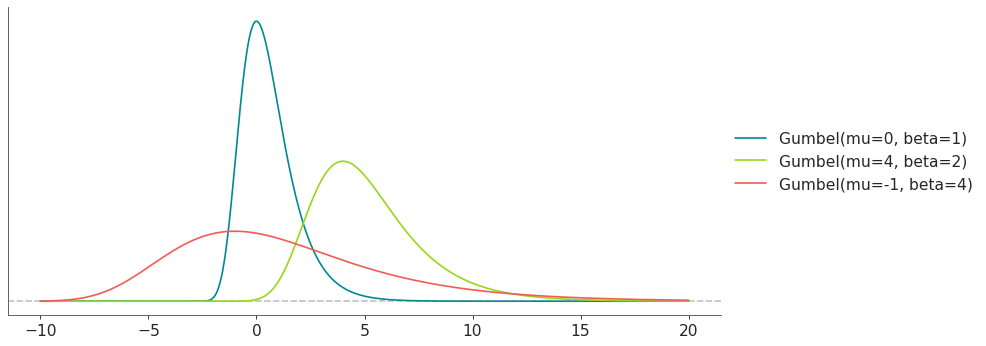

Support	$x \in \mathbb{R}$
Mean	$\mu + \beta\gamma$, where $\gamma$ is the Euler-Mascheroni constant
Variance	$\frac{\pi^2}{6} \beta^2$

Parameters:

mu (float) – Location parameter.
beta (float) – Scale parameter (beta > 0).

cdf(x)[source]#

Cumulative distribution function.

Parameters:: x (array_like) – Values on which to evaluate the cdf

entropy()[source]#: Entropy.

eti(mass=None, fmt='.2f')#

Equal-tailed interval containing mass.

Parameters:

mass (float) – Probability mass in the interval. Defaults to None,
used. (which results in the value of rcParams["stats.ci_prob"] being)
fmt (str) – fmt used to represent results using f-string fmt for floats. Default to “.2f” i.e. 2 digits after the decimal point. Use “none” for no format.

hdi(mass=None, fmt='.2f')#

Highest density interval containing mass.

Parameters:

mass (float) – Probability mass in the interval. Defaults to None,
used. (which results in the value of rcParams["stats.ci_prob"] being)
fmt (str) – fmt used to represent results using f-string fmt for floats. Default to “.2f” i.e. 2 digits after the decimal point. Use “none” for no format.

isf(x)#

Inverse survival function (inverse of sf).

Parameters:: x (array_like) – Values on which to evaluate the inverse of the sf

kurtosis()[source]#: Excess kurtosis.

lmoment1()[source]#: L-moment1 (mean).

lmoment2()[source]#: L-moment2 (l-scale).

lmoment3()[source]#: L-moment3 (l-skewness). This the ratio of L-moment3 to L-moment2.

lmoment4()[source]#: L-moment4 (l-kurtosis). This the ratio of L-moment4 to L-moment2.

lmoments(types='1234')#

Compute L-moments of the distribution.

Parameters:: types (str) – The type of moments to compute. Default is ‘1234’ where ‘1’ = L-moment1 (mean), ‘2’ = L-moment2 (l-scale), ‘3’ = L-moment3 (l-skewness), and ‘4’ = L-moment4 (l-kurtosis). To compute the standard deviation use ‘d’ Valid combinations are any subset of ‘1234’.

logcdf(x)#

Log cumulative distribution function.

Parameters:: x (array_like) – Values on which to evaluate the logcdf

logpdf(x)[source]#

Log probability density/mass function.

Parameters:: x (array_like) – Values on which to evaluate the logpdf

logsf(x)#

Log survival function log(1 - cdf).

Parameters:: x (array_like) – Values on which to evaluate the logsf

mean()[source]#: Mean.

median()[source]#: Median.

mode()[source]#: Mode.

moments(types='mvsk')#

Compute moments of the distribution.

It can also return the standard deviation

Parameters:: types (str) – The type of moments to compute. Default is ‘mvsk’ where ‘m’ = mean, ‘v’ = variance, ‘s’ = skewness, and ‘k’ = kurtosis. To compute the standard deviation use ‘d’ Valid combinations are any subset of ‘mvdsk’.

pdf(x)[source]#

Probability density/mass function.

Parameters:: x (array_like) – Values on which to evaluate the pdf

plot_cdf(moments=None, pointinterval=False, interval=None, levels=None, support='restricted', legend='legend', figsize=None, ax=None, **kwargs)#

Plot the cumulative distribution function.

Parameters:

moments (str) – Compute moments. Use any combination of the strings m, d, v, s or k for the mean (μ), standard deviation (σ), variance (σ²), skew (γ) or kurtosis (κ) respectively. Other strings will be ignored. Defaults to None.
pointinterval (bool) – Whether to include a plot of the quantiles. Defaults to False. If True the default is to plot the median and two interquantiles ranges.
interval (str) – Type of interval. Available options are highest density interval “hdi” (default), equal tailed interval “eti” or intervals defined by arbitrary “quantiles”. Defaults to the value in rcParams[“stats.ci_kind”].
levels (list) – Mass of the intervals. For hdi or eti the number of elements should be 2 or 1. For quantiles the number of elements should be 5, 3, 1 or 0 (in this last case nothing will be plotted).
support (str:) – If full use the finite end-points to set the limits of the plot. For unbounded end-points or if restricted use the 0.001 and 0.999 quantiles to set the limits.
legend (str) – Whether to include a string with the distribution and its parameter as a "legend" a "title" or not include them None.
figsize (tuple) – Size of the figure
ax (matplotlib axes)
kwargs (keyword arguments) – Additional keyword arguments passed to matplotlib plot function. For example, color, alpha, linewidth, etc.

plot_interactive(kind='pdf', xy_lim='both', pointinterval=True, interval=None, levels=None, figsize=None)#

Interactive exploration of distributions parameters.

Parameters:

kind (str:) – Type of plot. Available options are pdf, cdf and ppf.
xy_lim (str or tuple) – Set the limits of the x-axis and/or y-axis. Defaults to “both”, the limits of both axis are fixed. Use “auto” for automatic rescaling of x-axis and y-axis. Or set them manually by passing a tuple of 4 elements, the first two for x-axis, the last two for y-axis. The tuple can have None.
pointinterval (bool) – Whether to include a plot of the quantiles. Defaults to False. If True the default is to plot the median and two interquantiles ranges.
interval (str) – Type of interval. Available options are highest density interval “hdi” (default), equal tailed interval “eti” or intervals defined by arbitrary “quantiles”. Defaults to the value in rcParams[“stats.ci_kind”].
levels (list) – Mass of the intervals. For hdi or eti the number of elements should be 2 or 1. For quantiles the number of elements should be 5, 3, 1 or 0 (in this last case nothing will be plotted).
figsize (tuple) – Size of the figure

plot_isf(moments=None, pointinterval=False, interval=None, levels=None, legend='legend', figsize=None, ax=None, **kwargs)#

Plot the inverse survival function.

Parameters:

moments (str) – Compute moments. Use any combination of the strings m, d, v, s or k for the mean (μ), standard deviation (σ), variance (σ²), skew (γ) or kurtosis (κ) respectively. Other strings will be ignored. Defaults to None.
pointinterval (bool) – Whether to include a plot of the quantiles. Defaults to False. If True the default is to plot the median and two interquantiles ranges.
interval (str) – Type of interval. Available options are highest density interval “hdi” (default), equal tailed interval “eti” or intervals defined by arbitrary “quantiles”. Defaults to the value in rcParams[“stats.ci_kind”].
levels (list) – Mass of the intervals. For hdi or eti the number of elements should be 2 or 1. For quantiles the number of elements should be 5, 3, 1 or 0 (in this last case nothing will be plotted).
legend (str) – Whether to include a string with the distribution and its parameter as a "legend" a "title" or not include them None.
figsize (tuple) – Size of the figure
ax (matplotlib axes)

plot_pdf(moments=None, pointinterval=False, interval=None, levels=None, support='restricted', baseline=True, legend='legend', figsize=None, ax=None, **kwargs)#

Plot the pdf (continuous) or pmf (discrete).

Parameters:

moments (str) – Compute moments. Use any combination of the strings m, d, v, s or k for the mean (μ), standard deviation (σ), variance (σ²), skew (γ) or kurtosis (κ) respectively. Other strings will be ignored. Defaults to None.
pointinterval (bool) – Whether to include a plot of the quantiles. Defaults to False. If True the default is to plot the median and two interquantiles ranges.
interval (str) – Type of interval. Available options are highest density interval “hdi” (default), equal tailed interval “eti” or intervals defined by arbitrary “quantiles”. Defaults to the value in rcParams[“stats.ci_kind”].
levels (list) – Mass of the intervals. For hdi or eti the number of elements should be 2 or 1. For quantiles the number of elements should be 5, 3, 1 or 0 (in this last case nothing will be plotted).
support (str:) – If full use the finite end-points to set the limits of the plot. For unbounded end-points or if restricted use the 0.001 and 0.999 quantiles to set the limits.
baseline (bool) – Whether to include a horizontal line at y=0.
legend (str) – Whether to include a string with the distribution and its parameter as a "legend" a "title" or not include them None.
figsize (tuple) – Size of the figure
ax (matplotlib axes)
kwargs (keyword arguments) – Additional keyword arguments passed to matplotlib plot function. For example, color, alpha, linewidth, etc.

plot_ppf(moments=None, pointinterval=False, interval=None, levels=None, legend='legend', figsize=None, ax=None, **kwargs)#

Plot the quantile function.

Parameters:

moments (str) – Compute moments. Use any combination of the strings m, d, v, s or k for the mean (μ), standard deviation (σ), variance (σ²), skew (γ) or kurtosis (κ) respectively. Other strings will be ignored. Defaults to None.
pointinterval (bool) – Whether to include a plot of the quantiles. Defaults to False. If True the default is to plot the median and two interquantiles ranges.
interval (str) – Type of interval. Available options are highest density interval “hdi” (default), equal tailed interval “eti” or intervals defined by arbitrary “quantiles”. Defaults to the value in rcParams[“stats.ci_kind”].
levels (list) – Mass of the intervals. For hdi or eti the number of elements should be 2 or 1. For quantiles the number of elements should be 5, 3, 1 or 0 (in this last case nothing will be plotted).
legend (str) – Whether to include a string with the distribution and its parameter as a "legend" a "title" or not include them None.
figsize (tuple) – Size of the figure
ax (matplotlib axes)

plot_sf(moments=None, pointinterval=False, interval=None, levels=None, support='restricted', legend='legend', figsize=None, ax=None, **kwargs)#

Plot the survival distribution function (1 - CDF).

Parameters:

moments (str) – Compute moments. Use any combination of the strings m, d, v, s or k for the mean (μ), standard deviation (σ), variance (σ²), skew (γ) or kurtosis (κ) respectively. Other strings will be ignored. Defaults to None.
pointinterval (bool) – Whether to include a plot of the quantiles. Defaults to False. If True the default is to plot the median and two interquantiles ranges.
interval (str) – Type of interval. Available options are highest density interval “hdi” (default), equal tailed interval “eti” or intervals defined by arbitrary “quantiles”. Defaults to the value in rcParams[“stats.ci_kind”].
levels (list) – Mass of the intervals. For hdi or eti the number of elements should be 2 or 1. For quantiles the number of elements should be 5, 3, 1 or 0 (in this last case nothing will be plotted).
support (str:) – If full use the finite end-points to set the limits of the plot. For unbounded end-points or if restricted use the 0.001 and 0.999 quantiles to set the limits.
legend (str) – Whether to include a string with the distribution and its parameter as a "legend" a "title" or not include them None.
figsize (tuple) – Size of the figure
ax (matplotlib axes)
kwargs (keyword arguments) – Additional keyword arguments passed to matplotlib plot function. For example, color, alpha, linewidth, etc.

ppf(q)[source]#

Percent point function (inverse of cdf).

Parameters:: x (array_like) – Values on which to evaluate the inverse of the cdf

rvs(size=None, random_state=None)[source]#

Random sample.

Parameters:

size (int or tuple of ints, optional) – Defining number of random variates. Defaults to 1.
random_state ({None, int, numpy.random.Generator, numpy.random.RandomState}) – Defaults to None

sf(x)#

Survival function (1 - cdf).

Parameters:: x (array_like) – Values on which to evaluate the sf

skewness()[source]#: Skewness.

std()[source]#: Standard deviation.

summary(mass=None, interval=None, fmt='.2f')#

Namedtuple with the mean, median, sd, and lower and upper bounds.

Parameters:

mass (float) – Probability mass for the equal-tailed interval. Defaults to None,
used. (which results in the value of rcParams["stats.ci_prob"] being)
interval (str or list-like) – Type of interval. Available options are highest density interval “hdi”, equal tailed interval “eti” or arbitrary interval defined by a list-like object with a pair of values. Defaults to the value in rcParams[“stats.ci_kind”].
fmt (str) – fmt used to represent results using f-string fmt for floats. Default to “.2f” i.e. 2 digits after the decimal point.

to_bambi(**kwargs)#

Convert the PreliZ distribution to a Bambi Prior.

kwargsPyMC distributions properties: kwargs are used to specify properties such as shape or dims

Return type:: Bambi Prior

to_pymc(name=None, **kwargs)#

Convert the PreliZ distribution to a PyMC distribution.

namestr: Name of PyMC distribution. Needed if inside Model context
kwargsPyMC distributions properties: kwargs are used to specify properties such as shape or dims

Return type:: PyMC distribution

var()[source]#: Variance.

xvals(support, n_points=None)#

Provide x values in the support of the distribution.

This is useful for example when plotting.

Parameters:

support (str) – Available options are “full” or “restricted”. If “full” the values will cover the entire support of the distribution if the boundary is finite, or the quantiles 0.0001 or 0.9999, if infinite. If “restricted” the values will cover the quantile 0.0001 to 0.9999.
n_points (int) – Number of values to return. Defaults to 1000 for continuous distributions and 200 for discrete ones. For discrete distributions the returned values may be fewer than n_points if the actual number of discrete values in the support of the distribution is smaller than n_points.

class preliz.distributions.halfcauchy.HalfCauchy(beta=None)[source]#

HalfCauchy Distribution.

The pdf of this distribution is

\[f(x \mid \beta) = \frac{2}{\pi \beta [1 + (\frac{x}{\beta})^2]}\]

(Source code, png, hires.png, pdf)

Support	$x \in [0, \infty)$
Mean	undefined
Variance	undefined

Parameters:: beta (float) – Scale parameter $\beta$ (beta > 0)

cdf(x)[source]#

Cumulative distribution function.

Parameters:: x (array_like) – Values on which to evaluate the cdf

entropy()[source]#: Entropy.

eti(mass=None, fmt='.2f')#

Equal-tailed interval containing mass.

Parameters:

mass (float) – Probability mass in the interval. Defaults to None,
used. (which results in the value of rcParams["stats.ci_prob"] being)
fmt (str) – fmt used to represent results using f-string fmt for floats. Default to “.2f” i.e. 2 digits after the decimal point. Use “none” for no format.

hdi(mass=None, fmt='.2f')#

Highest density interval containing mass.

Parameters:

mass (float) – Probability mass in the interval. Defaults to None,
used. (which results in the value of rcParams["stats.ci_prob"] being)
fmt (str) – fmt used to represent results using f-string fmt for floats. Default to “.2f” i.e. 2 digits after the decimal point. Use “none” for no format.

isf(x)#

Inverse survival function (inverse of sf).

Parameters:: x (array_like) – Values on which to evaluate the inverse of the sf

kurtosis()[source]#: Excess kurtosis.

lmoment1()[source]#: L-moment1 (mean).

lmoment2()[source]#: L-moment2 (l-scale).

lmoment3()[source]#: L-moment3 (l-skewness). This the ratio of L-moment3 to L-moment2.

lmoment4()[source]#: L-moment4 (l-kurtosis). This the ratio of L-moment4 to L-moment2.

lmoments(types='1234')#

Compute L-moments of the distribution.

Parameters:: types (str) – The type of moments to compute. Default is ‘1234’ where ‘1’ = L-moment1 (mean), ‘2’ = L-moment2 (l-scale), ‘3’ = L-moment3 (l-skewness), and ‘4’ = L-moment4 (l-kurtosis). To compute the standard deviation use ‘d’ Valid combinations are any subset of ‘1234’.

logcdf(x)#

Log cumulative distribution function.

Parameters:: x (array_like) – Values on which to evaluate the logcdf

logpdf(x)[source]#

Log probability density/mass function.

Parameters:: x (array_like) – Values on which to evaluate the logpdf

logsf(x)#

Log survival function log(1 - cdf).

Parameters:: x (array_like) – Values on which to evaluate the logsf

mean()[source]#: Mean.

median()[source]#: Median.

mode()[source]#: Mode.

moments(types='mvsk')#

Compute moments of the distribution.

It can also return the standard deviation

Parameters:: types (str) – The type of moments to compute. Default is ‘mvsk’ where ‘m’ = mean, ‘v’ = variance, ‘s’ = skewness, and ‘k’ = kurtosis. To compute the standard deviation use ‘d’ Valid combinations are any subset of ‘mvdsk’.

pdf(x)[source]#

Probability density/mass function.

Parameters:: x (array_like) – Values on which to evaluate the pdf

plot_cdf(moments=None, pointinterval=False, interval=None, levels=None, support='restricted', legend='legend', figsize=None, ax=None, **kwargs)#

Plot the cumulative distribution function.

Parameters:

moments (str) – Compute moments. Use any combination of the strings m, d, v, s or k for the mean (μ), standard deviation (σ), variance (σ²), skew (γ) or kurtosis (κ) respectively. Other strings will be ignored. Defaults to None.
pointinterval (bool) – Whether to include a plot of the quantiles. Defaults to False. If True the default is to plot the median and two interquantiles ranges.
interval (str) – Type of interval. Available options are highest density interval “hdi” (default), equal tailed interval “eti” or intervals defined by arbitrary “quantiles”. Defaults to the value in rcParams[“stats.ci_kind”].
levels (list) – Mass of the intervals. For hdi or eti the number of elements should be 2 or 1. For quantiles the number of elements should be 5, 3, 1 or 0 (in this last case nothing will be plotted).
support (str:) – If full use the finite end-points to set the limits of the plot. For unbounded end-points or if restricted use the 0.001 and 0.999 quantiles to set the limits.
legend (str) – Whether to include a string with the distribution and its parameter as a "legend" a "title" or not include them None.
figsize (tuple) – Size of the figure
ax (matplotlib axes)
kwargs (keyword arguments) – Additional keyword arguments passed to matplotlib plot function. For example, color, alpha, linewidth, etc.

plot_interactive(kind='pdf', xy_lim='both', pointinterval=True, interval=None, levels=None, figsize=None)#

Interactive exploration of distributions parameters.

Parameters:

kind (str:) – Type of plot. Available options are pdf, cdf and ppf.
xy_lim (str or tuple) – Set the limits of the x-axis and/or y-axis. Defaults to “both”, the limits of both axis are fixed. Use “auto” for automatic rescaling of x-axis and y-axis. Or set them manually by passing a tuple of 4 elements, the first two for x-axis, the last two for y-axis. The tuple can have None.
pointinterval (bool) – Whether to include a plot of the quantiles. Defaults to False. If True the default is to plot the median and two interquantiles ranges.
interval (str) – Type of interval. Available options are highest density interval “hdi” (default), equal tailed interval “eti” or intervals defined by arbitrary “quantiles”. Defaults to the value in rcParams[“stats.ci_kind”].
levels (list) – Mass of the intervals. For hdi or eti the number of elements should be 2 or 1. For quantiles the number of elements should be 5, 3, 1 or 0 (in this last case nothing will be plotted).
figsize (tuple) – Size of the figure

plot_isf(moments=None, pointinterval=False, interval=None, levels=None, legend='legend', figsize=None, ax=None, **kwargs)#

Plot the inverse survival function.

Parameters:

moments (str) – Compute moments. Use any combination of the strings m, d, v, s or k for the mean (μ), standard deviation (σ), variance (σ²), skew (γ) or kurtosis (κ) respectively. Other strings will be ignored. Defaults to None.
pointinterval (bool) – Whether to include a plot of the quantiles. Defaults to False. If True the default is to plot the median and two interquantiles ranges.
interval (str) – Type of interval. Available options are highest density interval “hdi” (default), equal tailed interval “eti” or intervals defined by arbitrary “quantiles”. Defaults to the value in rcParams[“stats.ci_kind”].
levels (list) – Mass of the intervals. For hdi or eti the number of elements should be 2 or 1. For quantiles the number of elements should be 5, 3, 1 or 0 (in this last case nothing will be plotted).
legend (str) – Whether to include a string with the distribution and its parameter as a "legend" a "title" or not include them None.
figsize (tuple) – Size of the figure
ax (matplotlib axes)

plot_pdf(moments=None, pointinterval=False, interval=None, levels=None, support='restricted', baseline=True, legend='legend', figsize=None, ax=None, **kwargs)#

Plot the pdf (continuous) or pmf (discrete).

Parameters:

moments (str) – Compute moments. Use any combination of the strings m, d, v, s or k for the mean (μ), standard deviation (σ), variance (σ²), skew (γ) or kurtosis (κ) respectively. Other strings will be ignored. Defaults to None.
pointinterval (bool) – Whether to include a plot of the quantiles. Defaults to False. If True the default is to plot the median and two interquantiles ranges.
interval (str) – Type of interval. Available options are highest density interval “hdi” (default), equal tailed interval “eti” or intervals defined by arbitrary “quantiles”. Defaults to the value in rcParams[“stats.ci_kind”].
levels (list) – Mass of the intervals. For hdi or eti the number of elements should be 2 or 1. For quantiles the number of elements should be 5, 3, 1 or 0 (in this last case nothing will be plotted).
support (str:) – If full use the finite end-points to set the limits of the plot. For unbounded end-points or if restricted use the 0.001 and 0.999 quantiles to set the limits.
baseline (bool) – Whether to include a horizontal line at y=0.
legend (str) – Whether to include a string with the distribution and its parameter as a "legend" a "title" or not include them None.
figsize (tuple) – Size of the figure
ax (matplotlib axes)
kwargs (keyword arguments) – Additional keyword arguments passed to matplotlib plot function. For example, color, alpha, linewidth, etc.

plot_ppf(moments=None, pointinterval=False, interval=None, levels=None, legend='legend', figsize=None, ax=None, **kwargs)#

Plot the quantile function.

Parameters:

moments (str) – Compute moments. Use any combination of the strings m, d, v, s or k for the mean (μ), standard deviation (σ), variance (σ²), skew (γ) or kurtosis (κ) respectively. Other strings will be ignored. Defaults to None.
pointinterval (bool) – Whether to include a plot of the quantiles. Defaults to False. If True the default is to plot the median and two interquantiles ranges.
interval (str) – Type of interval. Available options are highest density interval “hdi” (default), equal tailed interval “eti” or intervals defined by arbitrary “quantiles”. Defaults to the value in rcParams[“stats.ci_kind”].
levels (list) – Mass of the intervals. For hdi or eti the number of elements should be 2 or 1. For quantiles the number of elements should be 5, 3, 1 or 0 (in this last case nothing will be plotted).
legend (str) – Whether to include a string with the distribution and its parameter as a "legend" a "title" or not include them None.
figsize (tuple) – Size of the figure
ax (matplotlib axes)

plot_sf(moments=None, pointinterval=False, interval=None, levels=None, support='restricted', legend='legend', figsize=None, ax=None, **kwargs)#

Plot the survival distribution function (1 - CDF).

Parameters:

moments (str) – Compute moments. Use any combination of the strings m, d, v, s or k for the mean (μ), standard deviation (σ), variance (σ²), skew (γ) or kurtosis (κ) respectively. Other strings will be ignored. Defaults to None.
pointinterval (bool) – Whether to include a plot of the quantiles. Defaults to False. If True the default is to plot the median and two interquantiles ranges.
interval (str) – Type of interval. Available options are highest density interval “hdi” (default), equal tailed interval “eti” or intervals defined by arbitrary “quantiles”. Defaults to the value in rcParams[“stats.ci_kind”].
levels (list) – Mass of the intervals. For hdi or eti the number of elements should be 2 or 1. For quantiles the number of elements should be 5, 3, 1 or 0 (in this last case nothing will be plotted).
support (str:) – If full use the finite end-points to set the limits of the plot. For unbounded end-points or if restricted use the 0.001 and 0.999 quantiles to set the limits.
legend (str) – Whether to include a string with the distribution and its parameter as a "legend" a "title" or not include them None.
figsize (tuple) – Size of the figure
ax (matplotlib axes)
kwargs (keyword arguments) – Additional keyword arguments passed to matplotlib plot function. For example, color, alpha, linewidth, etc.

ppf(q)[source]#

Percent point function (inverse of cdf).

Parameters:: x (array_like) – Values on which to evaluate the inverse of the cdf

rvs(size=None, random_state=None)[source]#

Random sample.

Parameters:

size (int or tuple of ints, optional) – Defining number of random variates. Defaults to 1.
random_state ({None, int, numpy.random.Generator, numpy.random.RandomState}) – Defaults to None

sf(x)#

Survival function (1 - cdf).

Parameters:: x (array_like) – Values on which to evaluate the sf

skewness()[source]#: Skewness.

std()[source]#: Standard deviation.

summary(mass=None, interval=None, fmt='.2f')#

Namedtuple with the mean, median, sd, and lower and upper bounds.

Parameters:

mass (float) – Probability mass for the equal-tailed interval. Defaults to None,
used. (which results in the value of rcParams["stats.ci_prob"] being)
interval (str or list-like) – Type of interval. Available options are highest density interval “hdi”, equal tailed interval “eti” or arbitrary interval defined by a list-like object with a pair of values. Defaults to the value in rcParams[“stats.ci_kind”].
fmt (str) – fmt used to represent results using f-string fmt for floats. Default to “.2f” i.e. 2 digits after the decimal point.

to_bambi(**kwargs)#

Convert the PreliZ distribution to a Bambi Prior.

kwargsPyMC distributions properties: kwargs are used to specify properties such as shape or dims

Return type:: Bambi Prior

to_pymc(name=None, **kwargs)#

Convert the PreliZ distribution to a PyMC distribution.

namestr: Name of PyMC distribution. Needed if inside Model context
kwargsPyMC distributions properties: kwargs are used to specify properties such as shape or dims

Return type:: PyMC distribution

var()[source]#: Variance.

xvals(support, n_points=None)#

Provide x values in the support of the distribution.

This is useful for example when plotting.

Parameters:

support (str) – Available options are “full” or “restricted”. If “full” the values will cover the entire support of the distribution if the boundary is finite, or the quantiles 0.0001 or 0.9999, if infinite. If “restricted” the values will cover the quantile 0.0001 to 0.9999.
n_points (int) – Number of values to return. Defaults to 1000 for continuous distributions and 200 for discrete ones. For discrete distributions the returned values may be fewer than n_points if the actual number of discrete values in the support of the distribution is smaller than n_points.

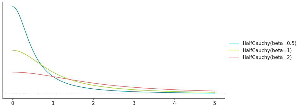
class preliz.distributions.halfnormal.HalfNormal(sigma=None, tau=None)[source]#

HalfNormal Distribution.

The pdf of this distribution is

\[f(x \mid \sigma) = \sqrt{\frac{2}{\pi\sigma^2}} \exp\left(\frac{-x^2}{2\sigma^2}\right)\]

(Source code, png, hires.png, pdf)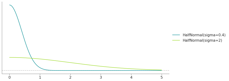

Support	$x \in [0, \infty)$
Mean	$\dfrac{\sigma \sqrt{2}}{\sqrt{\pi}}$
Variance	$\sigma^2\left(1 - \dfrac{2}{\pi}\right)$

HalfNormal distribution has 2 alternative parameterizations. In terms of sigma (standard deviation) or tau (precision).

The link between the 2 alternatives is given by

\[\tau = \frac{1}{\sigma^2}\]

Parameters:

sigma (float) – Scale parameter $\sigma$ (sigma > 0).
tau (float) – Precision $\tau$ (tau > 0).

cdf(x)[source]#

Cumulative distribution function.

Parameters:: x (array_like) – Values on which to evaluate the cdf

entropy()[source]#: Entropy.

eti(mass=None, fmt='.2f')#

Equal-tailed interval containing mass.

Parameters:

mass (float) – Probability mass in the interval. Defaults to None,
used. (which results in the value of rcParams["stats.ci_prob"] being)
fmt (str) – fmt used to represent results using f-string fmt for floats. Default to “.2f” i.e. 2 digits after the decimal point. Use “none” for no format.

hdi(mass=None, fmt='.2f')#

Highest density interval containing mass.

Parameters:

mass (float) – Probability mass in the interval. Defaults to None,
used. (which results in the value of rcParams["stats.ci_prob"] being)
fmt (str) – fmt used to represent results using f-string fmt for floats. Default to “.2f” i.e. 2 digits after the decimal point. Use “none” for no format.

isf(x)#

Inverse survival function (inverse of sf).

Parameters:: x (array_like) – Values on which to evaluate the inverse of the sf

kurtosis()[source]#: Excess kurtosis.

lmoment1()[source]#: L-moment1 (mean).

lmoment2()[source]#: L-moment2 (l-scale).

lmoment3()[source]#: L-moment3 (l-skewness). This the ratio of L-moment3 to L-moment2.

lmoment4()[source]#: L-moment4 (l-kurtosis). This the ratio of L-moment4 to L-moment2.

lmoments(types='1234')#

Compute L-moments of the distribution.

Parameters:: types (str) – The type of moments to compute. Default is ‘1234’ where ‘1’ = L-moment1 (mean), ‘2’ = L-moment2 (l-scale), ‘3’ = L-moment3 (l-skewness), and ‘4’ = L-moment4 (l-kurtosis). To compute the standard deviation use ‘d’ Valid combinations are any subset of ‘1234’.

logcdf(x)#

Log cumulative distribution function.

Parameters:: x (array_like) – Values on which to evaluate the logcdf

logpdf(x)[source]#

Log probability density/mass function.

Parameters:: x (array_like) – Values on which to evaluate the logpdf

logsf(x)#

Log survival function log(1 - cdf).

Parameters:: x (array_like) – Values on which to evaluate the logsf

mean()[source]#: Mean.

median()[source]#: Median.

mode()[source]#: Mode.

moments(types='mvsk')#

Compute moments of the distribution.

It can also return the standard deviation

Parameters:: types (str) – The type of moments to compute. Default is ‘mvsk’ where ‘m’ = mean, ‘v’ = variance, ‘s’ = skewness, and ‘k’ = kurtosis. To compute the standard deviation use ‘d’ Valid combinations are any subset of ‘mvdsk’.

pdf(x)[source]#

Probability density/mass function.

Parameters:: x (array_like) – Values on which to evaluate the pdf

plot_cdf(moments=None, pointinterval=False, interval=None, levels=None, support='restricted', legend='legend', figsize=None, ax=None, **kwargs)#

Plot the cumulative distribution function.

Parameters:

moments (str) – Compute moments. Use any combination of the strings m, d, v, s or k for the mean (μ), standard deviation (σ), variance (σ²), skew (γ) or kurtosis (κ) respectively. Other strings will be ignored. Defaults to None.
pointinterval (bool) – Whether to include a plot of the quantiles. Defaults to False. If True the default is to plot the median and two interquantiles ranges.
interval (str) – Type of interval. Available options are highest density interval “hdi” (default), equal tailed interval “eti” or intervals defined by arbitrary “quantiles”. Defaults to the value in rcParams[“stats.ci_kind”].
levels (list) – Mass of the intervals. For hdi or eti the number of elements should be 2 or 1. For quantiles the number of elements should be 5, 3, 1 or 0 (in this last case nothing will be plotted).
support (str:) – If full use the finite end-points to set the limits of the plot. For unbounded end-points or if restricted use the 0.001 and 0.999 quantiles to set the limits.
legend (str) – Whether to include a string with the distribution and its parameter as a "legend" a "title" or not include them None.
figsize (tuple) – Size of the figure
ax (matplotlib axes)
kwargs (keyword arguments) – Additional keyword arguments passed to matplotlib plot function. For example, color, alpha, linewidth, etc.

plot_interactive(kind='pdf', xy_lim='both', pointinterval=True, interval=None, levels=None, figsize=None)#

Interactive exploration of distributions parameters.

Parameters:

kind (str:) – Type of plot. Available options are pdf, cdf and ppf.
xy_lim (str or tuple) – Set the limits of the x-axis and/or y-axis. Defaults to “both”, the limits of both axis are fixed. Use “auto” for automatic rescaling of x-axis and y-axis. Or set them manually by passing a tuple of 4 elements, the first two for x-axis, the last two for y-axis. The tuple can have None.
pointinterval (bool) – Whether to include a plot of the quantiles. Defaults to False. If True the default is to plot the median and two interquantiles ranges.
interval (str) – Type of interval. Available options are highest density interval “hdi” (default), equal tailed interval “eti” or intervals defined by arbitrary “quantiles”. Defaults to the value in rcParams[“stats.ci_kind”].
levels (list) – Mass of the intervals. For hdi or eti the number of elements should be 2 or 1. For quantiles the number of elements should be 5, 3, 1 or 0 (in this last case nothing will be plotted).
figsize (tuple) – Size of the figure

plot_isf(moments=None, pointinterval=False, interval=None, levels=None, legend='legend', figsize=None, ax=None, **kwargs)#

Plot the inverse survival function.

Parameters:

moments (str) – Compute moments. Use any combination of the strings m, d, v, s or k for the mean (μ), standard deviation (σ), variance (σ²), skew (γ) or kurtosis (κ) respectively. Other strings will be ignored. Defaults to None.
pointinterval (bool) – Whether to include a plot of the quantiles. Defaults to False. If True the default is to plot the median and two interquantiles ranges.
interval (str) – Type of interval. Available options are highest density interval “hdi” (default), equal tailed interval “eti” or intervals defined by arbitrary “quantiles”. Defaults to the value in rcParams[“stats.ci_kind”].
levels (list) – Mass of the intervals. For hdi or eti the number of elements should be 2 or 1. For quantiles the number of elements should be 5, 3, 1 or 0 (in this last case nothing will be plotted).
legend (str) – Whether to include a string with the distribution and its parameter as a "legend" a "title" or not include them None.
figsize (tuple) – Size of the figure
ax (matplotlib axes)

plot_pdf(moments=None, pointinterval=False, interval=None, levels=None, support='restricted', baseline=True, legend='legend', figsize=None, ax=None, **kwargs)#

Plot the pdf (continuous) or pmf (discrete).

Parameters:

moments (str) – Compute moments. Use any combination of the strings m, d, v, s or k for the mean (μ), standard deviation (σ), variance (σ²), skew (γ) or kurtosis (κ) respectively. Other strings will be ignored. Defaults to None.
pointinterval (bool) – Whether to include a plot of the quantiles. Defaults to False. If True the default is to plot the median and two interquantiles ranges.
interval (str) – Type of interval. Available options are highest density interval “hdi” (default), equal tailed interval “eti” or intervals defined by arbitrary “quantiles”. Defaults to the value in rcParams[“stats.ci_kind”].
levels (list) – Mass of the intervals. For hdi or eti the number of elements should be 2 or 1. For quantiles the number of elements should be 5, 3, 1 or 0 (in this last case nothing will be plotted).
support (str:) – If full use the finite end-points to set the limits of the plot. For unbounded end-points or if restricted use the 0.001 and 0.999 quantiles to set the limits.
baseline (bool) – Whether to include a horizontal line at y=0.
legend (str) – Whether to include a string with the distribution and its parameter as a "legend" a "title" or not include them None.
figsize (tuple) – Size of the figure
ax (matplotlib axes)
kwargs (keyword arguments) – Additional keyword arguments passed to matplotlib plot function. For example, color, alpha, linewidth, etc.

plot_ppf(moments=None, pointinterval=False, interval=None, levels=None, legend='legend', figsize=None, ax=None, **kwargs)#

Plot the quantile function.

Parameters:

moments (str) – Compute moments. Use any combination of the strings m, d, v, s or k for the mean (μ), standard deviation (σ), variance (σ²), skew (γ) or kurtosis (κ) respectively. Other strings will be ignored. Defaults to None.
pointinterval (bool) – Whether to include a plot of the quantiles. Defaults to False. If True the default is to plot the median and two interquantiles ranges.
interval (str) – Type of interval. Available options are highest density interval “hdi” (default), equal tailed interval “eti” or intervals defined by arbitrary “quantiles”. Defaults to the value in rcParams[“stats.ci_kind”].
levels (list) – Mass of the intervals. For hdi or eti the number of elements should be 2 or 1. For quantiles the number of elements should be 5, 3, 1 or 0 (in this last case nothing will be plotted).
legend (str) – Whether to include a string with the distribution and its parameter as a "legend" a "title" or not include them None.
figsize (tuple) – Size of the figure
ax (matplotlib axes)

plot_sf(moments=None, pointinterval=False, interval=None, levels=None, support='restricted', legend='legend', figsize=None, ax=None, **kwargs)#

Plot the survival distribution function (1 - CDF).

Parameters:

moments (str) – Compute moments. Use any combination of the strings m, d, v, s or k for the mean (μ), standard deviation (σ), variance (σ²), skew (γ) or kurtosis (κ) respectively. Other strings will be ignored. Defaults to None.
pointinterval (bool) – Whether to include a plot of the quantiles. Defaults to False. If True the default is to plot the median and two interquantiles ranges.
interval (str) – Type of interval. Available options are highest density interval “hdi” (default), equal tailed interval “eti” or intervals defined by arbitrary “quantiles”. Defaults to the value in rcParams[“stats.ci_kind”].
levels (list) – Mass of the intervals. For hdi or eti the number of elements should be 2 or 1. For quantiles the number of elements should be 5, 3, 1 or 0 (in this last case nothing will be plotted).
support (str:) – If full use the finite end-points to set the limits of the plot. For unbounded end-points or if restricted use the 0.001 and 0.999 quantiles to set the limits.
legend (str) – Whether to include a string with the distribution and its parameter as a "legend" a "title" or not include them None.
figsize (tuple) – Size of the figure
ax (matplotlib axes)
kwargs (keyword arguments) – Additional keyword arguments passed to matplotlib plot function. For example, color, alpha, linewidth, etc.

ppf(q)[source]#

Percent point function (inverse of cdf).

Parameters:: x (array_like) – Values on which to evaluate the inverse of the cdf

rvs(size=None, random_state=None)[source]#

Random sample.

Parameters:

size (int or tuple of ints, optional) – Defining number of random variates. Defaults to 1.
random_state ({None, int, numpy.random.Generator, numpy.random.RandomState}) – Defaults to None

sf(x)#

Survival function (1 - cdf).

Parameters:: x (array_like) – Values on which to evaluate the sf

skewness()[source]#: Skewness.

std()[source]#: Standard deviation.

summary(mass=None, interval=None, fmt='.2f')#

Namedtuple with the mean, median, sd, and lower and upper bounds.

Parameters:

mass (float) – Probability mass for the equal-tailed interval. Defaults to None,
used. (which results in the value of rcParams["stats.ci_prob"] being)
interval (str or list-like) – Type of interval. Available options are highest density interval “hdi”, equal tailed interval “eti” or arbitrary interval defined by a list-like object with a pair of values. Defaults to the value in rcParams[“stats.ci_kind”].
fmt (str) – fmt used to represent results using f-string fmt for floats. Default to “.2f” i.e. 2 digits after the decimal point.

to_bambi(**kwargs)#

Convert the PreliZ distribution to a Bambi Prior.

kwargsPyMC distributions properties: kwargs are used to specify properties such as shape or dims

Return type:: Bambi Prior

to_pymc(name=None, **kwargs)#

Convert the PreliZ distribution to a PyMC distribution.

namestr: Name of PyMC distribution. Needed if inside Model context
kwargsPyMC distributions properties: kwargs are used to specify properties such as shape or dims

Return type:: PyMC distribution

var()[source]#: Variance.

xvals(support, n_points=None)#

Provide x values in the support of the distribution.

This is useful for example when plotting.

Parameters:

support (str) – Available options are “full” or “restricted”. If “full” the values will cover the entire support of the distribution if the boundary is finite, or the quantiles 0.0001 or 0.9999, if infinite. If “restricted” the values will cover the quantile 0.0001 to 0.9999.
n_points (int) – Number of values to return. Defaults to 1000 for continuous distributions and 200 for discrete ones. For discrete distributions the returned values may be fewer than n_points if the actual number of discrete values in the support of the distribution is smaller than n_points.

class preliz.distributions.halfstudentt.HalfStudentT(nu=None, sigma=None, lam=None)[source]#

HalfStudentT Distribution.

The pdf of this distribution is

\[f(x \mid \sigma,\nu) = \frac{2\;\Gamma\left(\frac{\nu+1}{2}\right)} {\Gamma\left(\frac{\nu}{2}\right)\sqrt{\nu\pi\sigma^2}} \left(1+\frac{1}{\nu}\frac{x^2}{\sigma^2}\right)^{-\frac{\nu+1}{2}}\]

(Source code, png, hires.png, pdf)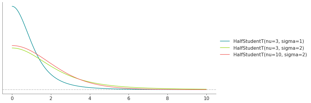

Support	$x \in [0, \infty)$
Mean	\[2\sigma\sqrt{\frac{\nu}{\pi}}\ \frac{\Gamma\left(\frac{\nu+1}{2}\right)} {\Gamma\left(\frac{\nu}{2}\right)(\nu-1)}\, \text{for } \nu > 2\]
Variance	\[\sigma^2\left(\frac{\nu}{\nu - 2}-\ \frac{4\nu}{\pi(\nu-1)^2}\left(\frac{\Gamma\left(\frac{\nu+1}{2}\right)} {\Gamma\left(\frac{\nu}{2}\right)}\right)^2\right) \text{for } \nu > 2\, \infty\ \text{for } 1 < \nu \le 2\, \text{otherwise undefined}\]

HalfStudentT distribution has 2 alternative parameterizations. In terms of nu and sigma (standard deviation as nu increases) or nu and lam (precision as nu increases).

The link between the 2 alternatives is given by

\[\lambda = \frac{1}{\sigma^2}\]

Parameters:

nu (float) – Degrees of freedom, also known as normality parameter (nu > 0).
sigma (float) – Scale parameter (sigma > 0). Converges to the standard deviation as nu increases.
lam (float) – Scale parameter (lam > 0). Converges to the precision as nu increases.

cdf(x)[source]#

Cumulative distribution function.

Parameters:: x (array_like) – Values on which to evaluate the cdf

entropy()[source]#: Entropy.

eti(mass=None, fmt='.2f')#

Equal-tailed interval containing mass.

Parameters:

mass (float) – Probability mass in the interval. Defaults to None,
used. (which results in the value of rcParams["stats.ci_prob"] being)
fmt (str) – fmt used to represent results using f-string fmt for floats. Default to “.2f” i.e. 2 digits after the decimal point. Use “none” for no format.

hdi(mass=None, fmt='.2f')#

Highest density interval containing mass.

Parameters:

mass (float) – Probability mass in the interval. Defaults to None,
used. (which results in the value of rcParams["stats.ci_prob"] being)
fmt (str) – fmt used to represent results using f-string fmt for floats. Default to “.2f” i.e. 2 digits after the decimal point. Use “none” for no format.

isf(x)#

Inverse survival function (inverse of sf).

Parameters:: x (array_like) – Values on which to evaluate the inverse of the sf

kurtosis()[source]#: Excess kurtosis.

lmoment1()[source]#: L-moment1 (mean).

lmoment2()[source]#: L-moment2 (l-scale).

lmoment3()[source]#: L-moment3 (l-skewness). This the ratio of L-moment3 to L-moment2.

lmoment4()[source]#: L-moment4 (l-kurtosis). This the ratio of L-moment4 to L-moment2.

lmoments(types='1234')#

Compute L-moments of the distribution.

Parameters:: types (str) – The type of moments to compute. Default is ‘1234’ where ‘1’ = L-moment1 (mean), ‘2’ = L-moment2 (l-scale), ‘3’ = L-moment3 (l-skewness), and ‘4’ = L-moment4 (l-kurtosis). To compute the standard deviation use ‘d’ Valid combinations are any subset of ‘1234’.

logcdf(x)#

Log cumulative distribution function.

Parameters:: x (array_like) – Values on which to evaluate the logcdf

logpdf(x)[source]#

Log probability density/mass function.

Parameters:: x (array_like) – Values on which to evaluate the logpdf

logsf(x)#

Log survival function log(1 - cdf).

Parameters:: x (array_like) – Values on which to evaluate the logsf

mean()[source]#: Mean.

median()[source]#: Median.

mode()[source]#: Mode.

moments(types='mvsk')#

Compute moments of the distribution.

It can also return the standard deviation

Parameters:: types (str) – The type of moments to compute. Default is ‘mvsk’ where ‘m’ = mean, ‘v’ = variance, ‘s’ = skewness, and ‘k’ = kurtosis. To compute the standard deviation use ‘d’ Valid combinations are any subset of ‘mvdsk’.

pdf(x)[source]#

Probability density/mass function.

Parameters:: x (array_like) – Values on which to evaluate the pdf

plot_cdf(moments=None, pointinterval=False, interval=None, levels=None, support='restricted', legend='legend', figsize=None, ax=None, **kwargs)#

Plot the cumulative distribution function.

Parameters:

moments (str) – Compute moments. Use any combination of the strings m, d, v, s or k for the mean (μ), standard deviation (σ), variance (σ²), skew (γ) or kurtosis (κ) respectively. Other strings will be ignored. Defaults to None.
pointinterval (bool) – Whether to include a plot of the quantiles. Defaults to False. If True the default is to plot the median and two interquantiles ranges.
interval (str) – Type of interval. Available options are highest density interval “hdi” (default), equal tailed interval “eti” or intervals defined by arbitrary “quantiles”. Defaults to the value in rcParams[“stats.ci_kind”].
levels (list) – Mass of the intervals. For hdi or eti the number of elements should be 2 or 1. For quantiles the number of elements should be 5, 3, 1 or 0 (in this last case nothing will be plotted).
support (str:) – If full use the finite end-points to set the limits of the plot. For unbounded end-points or if restricted use the 0.001 and 0.999 quantiles to set the limits.
legend (str) – Whether to include a string with the distribution and its parameter as a "legend" a "title" or not include them None.
figsize (tuple) – Size of the figure
ax (matplotlib axes)
kwargs (keyword arguments) – Additional keyword arguments passed to matplotlib plot function. For example, color, alpha, linewidth, etc.

plot_interactive(kind='pdf', xy_lim='both', pointinterval=True, interval=None, levels=None, figsize=None)#

Interactive exploration of distributions parameters.

Parameters:

kind (str:) – Type of plot. Available options are pdf, cdf and ppf.
xy_lim (str or tuple) – Set the limits of the x-axis and/or y-axis. Defaults to “both”, the limits of both axis are fixed. Use “auto” for automatic rescaling of x-axis and y-axis. Or set them manually by passing a tuple of 4 elements, the first two for x-axis, the last two for y-axis. The tuple can have None.
pointinterval (bool) – Whether to include a plot of the quantiles. Defaults to False. If True the default is to plot the median and two interquantiles ranges.
interval (str) – Type of interval. Available options are highest density interval “hdi” (default), equal tailed interval “eti” or intervals defined by arbitrary “quantiles”. Defaults to the value in rcParams[“stats.ci_kind”].
levels (list) – Mass of the intervals. For hdi or eti the number of elements should be 2 or 1. For quantiles the number of elements should be 5, 3, 1 or 0 (in this last case nothing will be plotted).
figsize (tuple) – Size of the figure

plot_isf(moments=None, pointinterval=False, interval=None, levels=None, legend='legend', figsize=None, ax=None, **kwargs)#

Plot the inverse survival function.

Parameters:

moments (str) – Compute moments. Use any combination of the strings m, d, v, s or k for the mean (μ), standard deviation (σ), variance (σ²), skew (γ) or kurtosis (κ) respectively. Other strings will be ignored. Defaults to None.
pointinterval (bool) – Whether to include a plot of the quantiles. Defaults to False. If True the default is to plot the median and two interquantiles ranges.
interval (str) – Type of interval. Available options are highest density interval “hdi” (default), equal tailed interval “eti” or intervals defined by arbitrary “quantiles”. Defaults to the value in rcParams[“stats.ci_kind”].
levels (list) – Mass of the intervals. For hdi or eti the number of elements should be 2 or 1. For quantiles the number of elements should be 5, 3, 1 or 0 (in this last case nothing will be plotted).
legend (str) – Whether to include a string with the distribution and its parameter as a "legend" a "title" or not include them None.
figsize (tuple) – Size of the figure
ax (matplotlib axes)

plot_pdf(moments=None, pointinterval=False, interval=None, levels=None, support='restricted', baseline=True, legend='legend', figsize=None, ax=None, **kwargs)#

Plot the pdf (continuous) or pmf (discrete).

Parameters:

moments (str) – Compute moments. Use any combination of the strings m, d, v, s or k for the mean (μ), standard deviation (σ), variance (σ²), skew (γ) or kurtosis (κ) respectively. Other strings will be ignored. Defaults to None.
pointinterval (bool) – Whether to include a plot of the quantiles. Defaults to False. If True the default is to plot the median and two interquantiles ranges.
interval (str) – Type of interval. Available options are highest density interval “hdi” (default), equal tailed interval “eti” or intervals defined by arbitrary “quantiles”. Defaults to the value in rcParams[“stats.ci_kind”].
levels (list) – Mass of the intervals. For hdi or eti the number of elements should be 2 or 1. For quantiles the number of elements should be 5, 3, 1 or 0 (in this last case nothing will be plotted).
support (str:) – If full use the finite end-points to set the limits of the plot. For unbounded end-points or if restricted use the 0.001 and 0.999 quantiles to set the limits.
baseline (bool) – Whether to include a horizontal line at y=0.
legend (str) – Whether to include a string with the distribution and its parameter as a "legend" a "title" or not include them None.
figsize (tuple) – Size of the figure
ax (matplotlib axes)
kwargs (keyword arguments) – Additional keyword arguments passed to matplotlib plot function. For example, color, alpha, linewidth, etc.

plot_ppf(moments=None, pointinterval=False, interval=None, levels=None, legend='legend', figsize=None, ax=None, **kwargs)#

Plot the quantile function.

Parameters:

moments (str) – Compute moments. Use any combination of the strings m, d, v, s or k for the mean (μ), standard deviation (σ), variance (σ²), skew (γ) or kurtosis (κ) respectively. Other strings will be ignored. Defaults to None.
pointinterval (bool) – Whether to include a plot of the quantiles. Defaults to False. If True the default is to plot the median and two interquantiles ranges.
interval (str) – Type of interval. Available options are highest density interval “hdi” (default), equal tailed interval “eti” or intervals defined by arbitrary “quantiles”. Defaults to the value in rcParams[“stats.ci_kind”].
levels (list) – Mass of the intervals. For hdi or eti the number of elements should be 2 or 1. For quantiles the number of elements should be 5, 3, 1 or 0 (in this last case nothing will be plotted).
legend (str) – Whether to include a string with the distribution and its parameter as a "legend" a "title" or not include them None.
figsize (tuple) – Size of the figure
ax (matplotlib axes)

plot_sf(moments=None, pointinterval=False, interval=None, levels=None, support='restricted', legend='legend', figsize=None, ax=None, **kwargs)#

Plot the survival distribution function (1 - CDF).

Parameters:

moments (str) – Compute moments. Use any combination of the strings m, d, v, s or k for the mean (μ), standard deviation (σ), variance (σ²), skew (γ) or kurtosis (κ) respectively. Other strings will be ignored. Defaults to None.
pointinterval (bool) – Whether to include a plot of the quantiles. Defaults to False. If True the default is to plot the median and two interquantiles ranges.
interval (str) – Type of interval. Available options are highest density interval “hdi” (default), equal tailed interval “eti” or intervals defined by arbitrary “quantiles”. Defaults to the value in rcParams[“stats.ci_kind”].
levels (list) – Mass of the intervals. For hdi or eti the number of elements should be 2 or 1. For quantiles the number of elements should be 5, 3, 1 or 0 (in this last case nothing will be plotted).
support (str:) – If full use the finite end-points to set the limits of the plot. For unbounded end-points or if restricted use the 0.001 and 0.999 quantiles to set the limits.
legend (str) – Whether to include a string with the distribution and its parameter as a "legend" a "title" or not include them None.
figsize (tuple) – Size of the figure
ax (matplotlib axes)
kwargs (keyword arguments) – Additional keyword arguments passed to matplotlib plot function. For example, color, alpha, linewidth, etc.

ppf(q)[source]#

Percent point function (inverse of cdf).

Parameters:: x (array_like) – Values on which to evaluate the inverse of the cdf

rvs(size=None, random_state=None)[source]#

Random sample.

Parameters:

size (int or tuple of ints, optional) – Defining number of random variates. Defaults to 1.
random_state ({None, int, numpy.random.Generator, numpy.random.RandomState}) – Defaults to None

sf(x)#

Survival function (1 - cdf).

Parameters:: x (array_like) – Values on which to evaluate the sf

skewness()[source]#: Skewness.

std()[source]#: Standard deviation.

summary(mass=None, interval=None, fmt='.2f')#

Namedtuple with the mean, median, sd, and lower and upper bounds.

Parameters:

mass (float) – Probability mass for the equal-tailed interval. Defaults to None,
used. (which results in the value of rcParams["stats.ci_prob"] being)
interval (str or list-like) – Type of interval. Available options are highest density interval “hdi”, equal tailed interval “eti” or arbitrary interval defined by a list-like object with a pair of values. Defaults to the value in rcParams[“stats.ci_kind”].
fmt (str) – fmt used to represent results using f-string fmt for floats. Default to “.2f” i.e. 2 digits after the decimal point.

to_bambi(**kwargs)#

Convert the PreliZ distribution to a Bambi Prior.

kwargsPyMC distributions properties: kwargs are used to specify properties such as shape or dims

Return type:: Bambi Prior

to_pymc(name=None, **kwargs)#

Convert the PreliZ distribution to a PyMC distribution.

namestr: Name of PyMC distribution. Needed if inside Model context
kwargsPyMC distributions properties: kwargs are used to specify properties such as shape or dims

Return type:: PyMC distribution

var()[source]#: Variance.

xvals(support, n_points=None)#

Provide x values in the support of the distribution.

This is useful for example when plotting.

Parameters:

support (str) – Available options are “full” or “restricted”. If “full” the values will cover the entire support of the distribution if the boundary is finite, or the quantiles 0.0001 or 0.9999, if infinite. If “restricted” the values will cover the quantile 0.0001 to 0.9999.
n_points (int) – Number of values to return. Defaults to 1000 for continuous distributions and 200 for discrete ones. For discrete distributions the returned values may be fewer than n_points if the actual number of discrete values in the support of the distribution is smaller than n_points.

class preliz.distributions.inversegamma.InverseGamma(alpha=None, beta=None, mu=None, sigma=None)[source]#

Inverse gamma distribution, the reciprocal of the gamma distribution.

The pdf of this distribution is

\[f(x \mid \alpha, \beta) = \frac{\beta^{\alpha}}{\Gamma(\alpha)} x^{-\alpha - 1} \exp\left(\frac{-\beta}{x}\right)\]

(Source code, png, hires.png, pdf)

Support	$x \in (0, \infty)$
Mean	$\dfrac{\beta}{\alpha-1}$ for $\alpha > 1$
Variance	$\dfrac{\beta^2}{(\alpha-1)^2(\alpha - 2)}$ for $\alpha > 2$

Inverse gamma distribution has 2 alternative parameterization. In terms of alpha and beta or mu (mean) and sigma (standard deviation).

The link between the 2 alternatives is given by

\[\begin{split}\alpha &= \frac{\mu^2}{\sigma^2} + 2 \\ \beta &= \frac{\mu^3}{\sigma^2} + \mu\end{split}\]

Parameters:

alpha (float) – Shape parameter (alpha > 0).
beta (float) – Scale parameter (beta > 0).
mu (float) – Mean (mu > 0).
sigma (float) – Standard deviation (sigma > 0)

cdf(x)[source]#

Cumulative distribution function.

Parameters:: x (array_like) – Values on which to evaluate the cdf

entropy()[source]#: Entropy.

eti(mass=None, fmt='.2f')#

Equal-tailed interval containing mass.

Parameters:

mass (float) – Probability mass in the interval. Defaults to None,
used. (which results in the value of rcParams["stats.ci_prob"] being)
fmt (str) – fmt used to represent results using f-string fmt for floats. Default to “.2f” i.e. 2 digits after the decimal point. Use “none” for no format.

hdi(mass=None, fmt='.2f')#

Highest density interval containing mass.

Parameters:

mass (float) – Probability mass in the interval. Defaults to None,
used. (which results in the value of rcParams["stats.ci_prob"] being)
fmt (str) – fmt used to represent results using f-string fmt for floats. Default to “.2f” i.e. 2 digits after the decimal point. Use “none” for no format.

isf(x)#

Inverse survival function (inverse of sf).

Parameters:: x (array_like) – Values on which to evaluate the inverse of the sf

kurtosis()[source]#: Excess kurtosis.

lmoment1()[source]#: L-moment1 (mean).

lmoment2()[source]#: L-moment2 (l-scale).

lmoment3()[source]#: L-moment3 (l-skewness). This the ratio of L-moment3 to L-moment2.

lmoment4()[source]#: L-moment4 (l-kurtosis). This the ratio of L-moment4 to L-moment2.

lmoments(types='1234')#

Compute L-moments of the distribution.

Parameters:: types (str) – The type of moments to compute. Default is ‘1234’ where ‘1’ = L-moment1 (mean), ‘2’ = L-moment2 (l-scale), ‘3’ = L-moment3 (l-skewness), and ‘4’ = L-moment4 (l-kurtosis). To compute the standard deviation use ‘d’ Valid combinations are any subset of ‘1234’.

logcdf(x)#

Log cumulative distribution function.

Parameters:: x (array_like) – Values on which to evaluate the logcdf

logpdf(x)[source]#

Log probability density/mass function.

Parameters:: x (array_like) – Values on which to evaluate the logpdf

logsf(x)#

Log survival function log(1 - cdf).

Parameters:: x (array_like) – Values on which to evaluate the logsf

mean()[source]#: Mean.

median()[source]#: Median.

mode()[source]#: Mode.

moments(types='mvsk')#

Compute moments of the distribution.

It can also return the standard deviation

Parameters:: types (str) – The type of moments to compute. Default is ‘mvsk’ where ‘m’ = mean, ‘v’ = variance, ‘s’ = skewness, and ‘k’ = kurtosis. To compute the standard deviation use ‘d’ Valid combinations are any subset of ‘mvdsk’.

pdf(x)[source]#

Probability density/mass function.

Parameters:: x (array_like) – Values on which to evaluate the pdf

plot_cdf(moments=None, pointinterval=False, interval=None, levels=None, support='restricted', legend='legend', figsize=None, ax=None, **kwargs)#

Plot the cumulative distribution function.

Parameters:

moments (str) – Compute moments. Use any combination of the strings m, d, v, s or k for the mean (μ), standard deviation (σ), variance (σ²), skew (γ) or kurtosis (κ) respectively. Other strings will be ignored. Defaults to None.
pointinterval (bool) – Whether to include a plot of the quantiles. Defaults to False. If True the default is to plot the median and two interquantiles ranges.
interval (str) – Type of interval. Available options are highest density interval “hdi” (default), equal tailed interval “eti” or intervals defined by arbitrary “quantiles”. Defaults to the value in rcParams[“stats.ci_kind”].
levels (list) – Mass of the intervals. For hdi or eti the number of elements should be 2 or 1. For quantiles the number of elements should be 5, 3, 1 or 0 (in this last case nothing will be plotted).
support (str:) – If full use the finite end-points to set the limits of the plot. For unbounded end-points or if restricted use the 0.001 and 0.999 quantiles to set the limits.
legend (str) – Whether to include a string with the distribution and its parameter as a "legend" a "title" or not include them None.
figsize (tuple) – Size of the figure
ax (matplotlib axes)
kwargs (keyword arguments) – Additional keyword arguments passed to matplotlib plot function. For example, color, alpha, linewidth, etc.

plot_interactive(kind='pdf', xy_lim='both', pointinterval=True, interval=None, levels=None, figsize=None)#

Interactive exploration of distributions parameters.

Parameters:

kind (str:) – Type of plot. Available options are pdf, cdf and ppf.
xy_lim (str or tuple) – Set the limits of the x-axis and/or y-axis. Defaults to “both”, the limits of both axis are fixed. Use “auto” for automatic rescaling of x-axis and y-axis. Or set them manually by passing a tuple of 4 elements, the first two for x-axis, the last two for y-axis. The tuple can have None.
pointinterval (bool) – Whether to include a plot of the quantiles. Defaults to False. If True the default is to plot the median and two interquantiles ranges.
interval (str) – Type of interval. Available options are highest density interval “hdi” (default), equal tailed interval “eti” or intervals defined by arbitrary “quantiles”. Defaults to the value in rcParams[“stats.ci_kind”].
levels (list) – Mass of the intervals. For hdi or eti the number of elements should be 2 or 1. For quantiles the number of elements should be 5, 3, 1 or 0 (in this last case nothing will be plotted).
figsize (tuple) – Size of the figure

plot_isf(moments=None, pointinterval=False, interval=None, levels=None, legend='legend', figsize=None, ax=None, **kwargs)#

Plot the inverse survival function.

Parameters:

moments (str) – Compute moments. Use any combination of the strings m, d, v, s or k for the mean (μ), standard deviation (σ), variance (σ²), skew (γ) or kurtosis (κ) respectively. Other strings will be ignored. Defaults to None.
pointinterval (bool) – Whether to include a plot of the quantiles. Defaults to False. If True the default is to plot the median and two interquantiles ranges.
interval (str) – Type of interval. Available options are highest density interval “hdi” (default), equal tailed interval “eti” or intervals defined by arbitrary “quantiles”. Defaults to the value in rcParams[“stats.ci_kind”].
levels (list) – Mass of the intervals. For hdi or eti the number of elements should be 2 or 1. For quantiles the number of elements should be 5, 3, 1 or 0 (in this last case nothing will be plotted).
legend (str) – Whether to include a string with the distribution and its parameter as a "legend" a "title" or not include them None.
figsize (tuple) – Size of the figure
ax (matplotlib axes)

plot_pdf(moments=None, pointinterval=False, interval=None, levels=None, support='restricted', baseline=True, legend='legend', figsize=None, ax=None, **kwargs)#

Plot the pdf (continuous) or pmf (discrete).

Parameters:

moments (str) – Compute moments. Use any combination of the strings m, d, v, s or k for the mean (μ), standard deviation (σ), variance (σ²), skew (γ) or kurtosis (κ) respectively. Other strings will be ignored. Defaults to None.
pointinterval (bool) – Whether to include a plot of the quantiles. Defaults to False. If True the default is to plot the median and two interquantiles ranges.
interval (str) – Type of interval. Available options are highest density interval “hdi” (default), equal tailed interval “eti” or intervals defined by arbitrary “quantiles”. Defaults to the value in rcParams[“stats.ci_kind”].
levels (list) – Mass of the intervals. For hdi or eti the number of elements should be 2 or 1. For quantiles the number of elements should be 5, 3, 1 or 0 (in this last case nothing will be plotted).
support (str:) – If full use the finite end-points to set the limits of the plot. For unbounded end-points or if restricted use the 0.001 and 0.999 quantiles to set the limits.
baseline (bool) – Whether to include a horizontal line at y=0.
legend (str) – Whether to include a string with the distribution and its parameter as a "legend" a "title" or not include them None.
figsize (tuple) – Size of the figure
ax (matplotlib axes)
kwargs (keyword arguments) – Additional keyword arguments passed to matplotlib plot function. For example, color, alpha, linewidth, etc.

plot_ppf(moments=None, pointinterval=False, interval=None, levels=None, legend='legend', figsize=None, ax=None, **kwargs)#

Plot the quantile function.

Parameters:

moments (str) – Compute moments. Use any combination of the strings m, d, v, s or k for the mean (μ), standard deviation (σ), variance (σ²), skew (γ) or kurtosis (κ) respectively. Other strings will be ignored. Defaults to None.
pointinterval (bool) – Whether to include a plot of the quantiles. Defaults to False. If True the default is to plot the median and two interquantiles ranges.
interval (str) – Type of interval. Available options are highest density interval “hdi” (default), equal tailed interval “eti” or intervals defined by arbitrary “quantiles”. Defaults to the value in rcParams[“stats.ci_kind”].
levels (list) – Mass of the intervals. For hdi or eti the number of elements should be 2 or 1. For quantiles the number of elements should be 5, 3, 1 or 0 (in this last case nothing will be plotted).
legend (str) – Whether to include a string with the distribution and its parameter as a "legend" a "title" or not include them None.
figsize (tuple) – Size of the figure
ax (matplotlib axes)

plot_sf(moments=None, pointinterval=False, interval=None, levels=None, support='restricted', legend='legend', figsize=None, ax=None, **kwargs)#

Plot the survival distribution function (1 - CDF).

Parameters:

moments (str) – Compute moments. Use any combination of the strings m, d, v, s or k for the mean (μ), standard deviation (σ), variance (σ²), skew (γ) or kurtosis (κ) respectively. Other strings will be ignored. Defaults to None.
pointinterval (bool) – Whether to include a plot of the quantiles. Defaults to False. If True the default is to plot the median and two interquantiles ranges.
interval (str) – Type of interval. Available options are highest density interval “hdi” (default), equal tailed interval “eti” or intervals defined by arbitrary “quantiles”. Defaults to the value in rcParams[“stats.ci_kind”].
levels (list) – Mass of the intervals. For hdi or eti the number of elements should be 2 or 1. For quantiles the number of elements should be 5, 3, 1 or 0 (in this last case nothing will be plotted).
support (str:) – If full use the finite end-points to set the limits of the plot. For unbounded end-points or if restricted use the 0.001 and 0.999 quantiles to set the limits.
legend (str) – Whether to include a string with the distribution and its parameter as a "legend" a "title" or not include them None.
figsize (tuple) – Size of the figure
ax (matplotlib axes)
kwargs (keyword arguments) – Additional keyword arguments passed to matplotlib plot function. For example, color, alpha, linewidth, etc.

ppf(q)[source]#

Percent point function (inverse of cdf).

Parameters:: x (array_like) – Values on which to evaluate the inverse of the cdf

rvs(size=None, random_state=None)[source]#

Random sample.

Parameters:

size (int or tuple of ints, optional) – Defining number of random variates. Defaults to 1.
random_state ({None, int, numpy.random.Generator, numpy.random.RandomState}) – Defaults to None

sf(x)#

Survival function (1 - cdf).

Parameters:: x (array_like) – Values on which to evaluate the sf

skewness()[source]#: Skewness.

std()[source]#: Standard deviation.

summary(mass=None, interval=None, fmt='.2f')#

Namedtuple with the mean, median, sd, and lower and upper bounds.

Parameters:

mass (float) – Probability mass for the equal-tailed interval. Defaults to None,
used. (which results in the value of rcParams["stats.ci_prob"] being)
interval (str or list-like) – Type of interval. Available options are highest density interval “hdi”, equal tailed interval “eti” or arbitrary interval defined by a list-like object with a pair of values. Defaults to the value in rcParams[“stats.ci_kind”].
fmt (str) – fmt used to represent results using f-string fmt for floats. Default to “.2f” i.e. 2 digits after the decimal point.

to_bambi(**kwargs)#

Convert the PreliZ distribution to a Bambi Prior.

kwargsPyMC distributions properties: kwargs are used to specify properties such as shape or dims

Return type:: Bambi Prior

to_pymc(name=None, **kwargs)#

Convert the PreliZ distribution to a PyMC distribution.

namestr: Name of PyMC distribution. Needed if inside Model context
kwargsPyMC distributions properties: kwargs are used to specify properties such as shape or dims

Return type:: PyMC distribution

var()[source]#: Variance.

xvals(support, n_points=None)#

Provide x values in the support of the distribution.

This is useful for example when plotting.

Parameters:

support (str) – Available options are “full” or “restricted”. If “full” the values will cover the entire support of the distribution if the boundary is finite, or the quantiles 0.0001 or 0.9999, if infinite. If “restricted” the values will cover the quantile 0.0001 to 0.9999.
n_points (int) – Number of values to return. Defaults to 1000 for continuous distributions and 200 for discrete ones. For discrete distributions the returned values may be fewer than n_points if the actual number of discrete values in the support of the distribution is smaller than n_points.

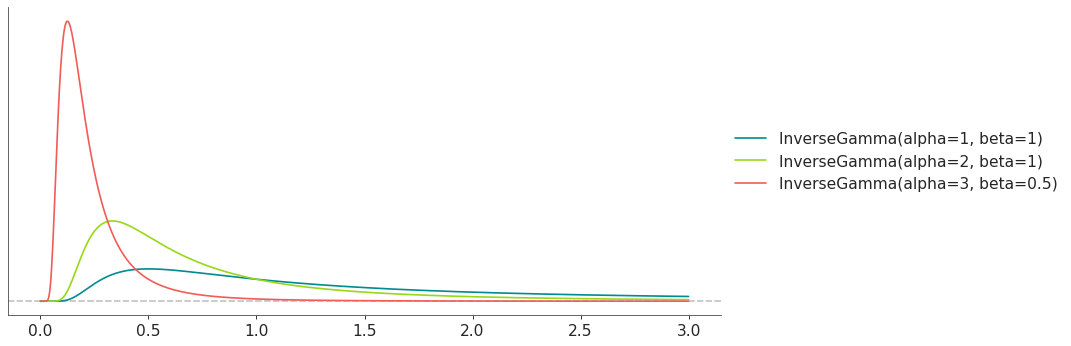
class preliz.distributions.kumaraswamy.Kumaraswamy(a=None, b=None)[source]#

Kumaraswamy distribution.

The pdf of this distribution is

\[f(x \mid a, b) = a b x^{a - 1} (1 - x^a)^{b - 1}\]

(Source code, png, hires.png, pdf)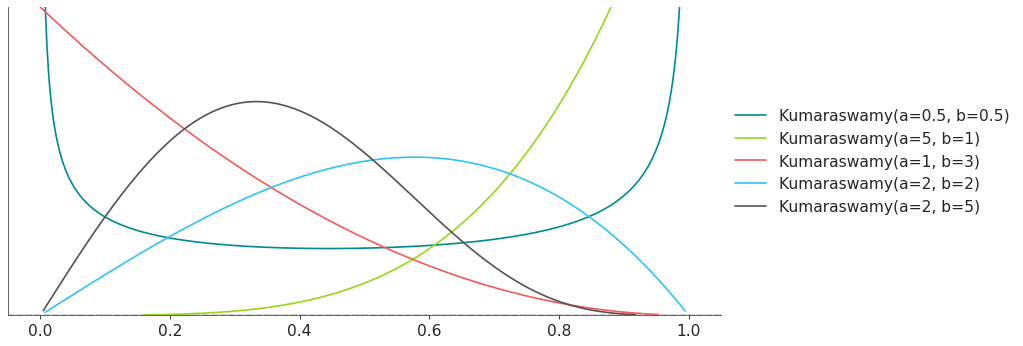

Support	$x \in (0, 1)$
Mean	$b B(1 + \tfrac{1}{a}, b)$
Variance	$b B(1 + \tfrac{2}{a}, b) - (b B(1 + \tfrac{1}{a}, b))^2$

Parameters:

a (float) – a > 0.
b (float) – b > 0.

cdf(x)[source]#

Cumulative distribution function.

Parameters:: x (array_like) – Values on which to evaluate the cdf

entropy()[source]#: Entropy.

eti(mass=None, fmt='.2f')#

Equal-tailed interval containing mass.

Parameters:

mass (float) – Probability mass in the interval. Defaults to None,
used. (which results in the value of rcParams["stats.ci_prob"] being)
fmt (str) – fmt used to represent results using f-string fmt for floats. Default to “.2f” i.e. 2 digits after the decimal point. Use “none” for no format.

hdi(mass=None, fmt='.2f')#

Highest density interval containing mass.

Parameters:

mass (float) – Probability mass in the interval. Defaults to None,
used. (which results in the value of rcParams["stats.ci_prob"] being)
fmt (str) – fmt used to represent results using f-string fmt for floats. Default to “.2f” i.e. 2 digits after the decimal point. Use “none” for no format.

isf(x)#

Inverse survival function (inverse of sf).

Parameters:: x (array_like) – Values on which to evaluate the inverse of the sf

kurtosis()[source]#: Excess kurtosis.

lmoment1()[source]#: L-moment1 (mean).

lmoment2()[source]#: L-moment2 (l-scale).

lmoment3()[source]#: L-moment3 (l-skewness). This the ratio of L-moment3 to L-moment2.

lmoment4()[source]#: L-moment4 (l-kurtosis). This the ratio of L-moment4 to L-moment2.

lmoments(types='1234')#

Compute L-moments of the distribution.

Parameters:: types (str) – The type of moments to compute. Default is ‘1234’ where ‘1’ = L-moment1 (mean), ‘2’ = L-moment2 (l-scale), ‘3’ = L-moment3 (l-skewness), and ‘4’ = L-moment4 (l-kurtosis). To compute the standard deviation use ‘d’ Valid combinations are any subset of ‘1234’.

logcdf(x)#

Log cumulative distribution function.

Parameters:: x (array_like) – Values on which to evaluate the logcdf

logpdf(x)[source]#

Log probability density/mass function.

Parameters:: x (array_like) – Values on which to evaluate the logpdf

logsf(x)#

Log survival function log(1 - cdf).

Parameters:: x (array_like) – Values on which to evaluate the logsf

mean()[source]#: Mean.

median()[source]#: Median.

mode()[source]#: Mode.

moments(types='mvsk')#

Compute moments of the distribution.

It can also return the standard deviation

Parameters:: types (str) – The type of moments to compute. Default is ‘mvsk’ where ‘m’ = mean, ‘v’ = variance, ‘s’ = skewness, and ‘k’ = kurtosis. To compute the standard deviation use ‘d’ Valid combinations are any subset of ‘mvdsk’.

pdf(x)[source]#

Probability density/mass function.

Parameters:: x (array_like) – Values on which to evaluate the pdf

plot_cdf(moments=None, pointinterval=False, interval=None, levels=None, support='restricted', legend='legend', figsize=None, ax=None, **kwargs)#

Plot the cumulative distribution function.

Parameters:

moments (str) – Compute moments. Use any combination of the strings m, d, v, s or k for the mean (μ), standard deviation (σ), variance (σ²), skew (γ) or kurtosis (κ) respectively. Other strings will be ignored. Defaults to None.
pointinterval (bool) – Whether to include a plot of the quantiles. Defaults to False. If True the default is to plot the median and two interquantiles ranges.
interval (str) – Type of interval. Available options are highest density interval “hdi” (default), equal tailed interval “eti” or intervals defined by arbitrary “quantiles”. Defaults to the value in rcParams[“stats.ci_kind”].
levels (list) – Mass of the intervals. For hdi or eti the number of elements should be 2 or 1. For quantiles the number of elements should be 5, 3, 1 or 0 (in this last case nothing will be plotted).
support (str:) – If full use the finite end-points to set the limits of the plot. For unbounded end-points or if restricted use the 0.001 and 0.999 quantiles to set the limits.
legend (str) – Whether to include a string with the distribution and its parameter as a "legend" a "title" or not include them None.
figsize (tuple) – Size of the figure
ax (matplotlib axes)
kwargs (keyword arguments) – Additional keyword arguments passed to matplotlib plot function. For example, color, alpha, linewidth, etc.

plot_interactive(kind='pdf', xy_lim='both', pointinterval=True, interval=None, levels=None, figsize=None)#

Interactive exploration of distributions parameters.

Parameters:

kind (str:) – Type of plot. Available options are pdf, cdf and ppf.
xy_lim (str or tuple) – Set the limits of the x-axis and/or y-axis. Defaults to “both”, the limits of both axis are fixed. Use “auto” for automatic rescaling of x-axis and y-axis. Or set them manually by passing a tuple of 4 elements, the first two for x-axis, the last two for y-axis. The tuple can have None.
pointinterval (bool) – Whether to include a plot of the quantiles. Defaults to False. If True the default is to plot the median and two interquantiles ranges.
interval (str) – Type of interval. Available options are highest density interval “hdi” (default), equal tailed interval “eti” or intervals defined by arbitrary “quantiles”. Defaults to the value in rcParams[“stats.ci_kind”].
levels (list) – Mass of the intervals. For hdi or eti the number of elements should be 2 or 1. For quantiles the number of elements should be 5, 3, 1 or 0 (in this last case nothing will be plotted).
figsize (tuple) – Size of the figure

plot_isf(moments=None, pointinterval=False, interval=None, levels=None, legend='legend', figsize=None, ax=None, **kwargs)#

Plot the inverse survival function.

Parameters:

moments (str) – Compute moments. Use any combination of the strings m, d, v, s or k for the mean (μ), standard deviation (σ), variance (σ²), skew (γ) or kurtosis (κ) respectively. Other strings will be ignored. Defaults to None.
pointinterval (bool) – Whether to include a plot of the quantiles. Defaults to False. If True the default is to plot the median and two interquantiles ranges.
interval (str) – Type of interval. Available options are highest density interval “hdi” (default), equal tailed interval “eti” or intervals defined by arbitrary “quantiles”. Defaults to the value in rcParams[“stats.ci_kind”].
levels (list) – Mass of the intervals. For hdi or eti the number of elements should be 2 or 1. For quantiles the number of elements should be 5, 3, 1 or 0 (in this last case nothing will be plotted).
legend (str) – Whether to include a string with the distribution and its parameter as a "legend" a "title" or not include them None.
figsize (tuple) – Size of the figure
ax (matplotlib axes)

plot_pdf(moments=None, pointinterval=False, interval=None, levels=None, support='restricted', baseline=True, legend='legend', figsize=None, ax=None, **kwargs)#

Plot the pdf (continuous) or pmf (discrete).

Parameters:

moments (str) – Compute moments. Use any combination of the strings m, d, v, s or k for the mean (μ), standard deviation (σ), variance (σ²), skew (γ) or kurtosis (κ) respectively. Other strings will be ignored. Defaults to None.
pointinterval (bool) – Whether to include a plot of the quantiles. Defaults to False. If True the default is to plot the median and two interquantiles ranges.
interval (str) – Type of interval. Available options are highest density interval “hdi” (default), equal tailed interval “eti” or intervals defined by arbitrary “quantiles”. Defaults to the value in rcParams[“stats.ci_kind”].
levels (list) – Mass of the intervals. For hdi or eti the number of elements should be 2 or 1. For quantiles the number of elements should be 5, 3, 1 or 0 (in this last case nothing will be plotted).
support (str:) – If full use the finite end-points to set the limits of the plot. For unbounded end-points or if restricted use the 0.001 and 0.999 quantiles to set the limits.
baseline (bool) – Whether to include a horizontal line at y=0.
legend (str) – Whether to include a string with the distribution and its parameter as a "legend" a "title" or not include them None.
figsize (tuple) – Size of the figure
ax (matplotlib axes)
kwargs (keyword arguments) – Additional keyword arguments passed to matplotlib plot function. For example, color, alpha, linewidth, etc.

plot_ppf(moments=None, pointinterval=False, interval=None, levels=None, legend='legend', figsize=None, ax=None, **kwargs)#

Plot the quantile function.

Parameters:

moments (str) – Compute moments. Use any combination of the strings m, d, v, s or k for the mean (μ), standard deviation (σ), variance (σ²), skew (γ) or kurtosis (κ) respectively. Other strings will be ignored. Defaults to None.
pointinterval (bool) – Whether to include a plot of the quantiles. Defaults to False. If True the default is to plot the median and two interquantiles ranges.
interval (str) – Type of interval. Available options are highest density interval “hdi” (default), equal tailed interval “eti” or intervals defined by arbitrary “quantiles”. Defaults to the value in rcParams[“stats.ci_kind”].
levels (list) – Mass of the intervals. For hdi or eti the number of elements should be 2 or 1. For quantiles the number of elements should be 5, 3, 1 or 0 (in this last case nothing will be plotted).
legend (str) – Whether to include a string with the distribution and its parameter as a "legend" a "title" or not include them None.
figsize (tuple) – Size of the figure
ax (matplotlib axes)

plot_sf(moments=None, pointinterval=False, interval=None, levels=None, support='restricted', legend='legend', figsize=None, ax=None, **kwargs)#

Plot the survival distribution function (1 - CDF).

Parameters:

moments (str) – Compute moments. Use any combination of the strings m, d, v, s or k for the mean (μ), standard deviation (σ), variance (σ²), skew (γ) or kurtosis (κ) respectively. Other strings will be ignored. Defaults to None.
pointinterval (bool) – Whether to include a plot of the quantiles. Defaults to False. If True the default is to plot the median and two interquantiles ranges.
interval (str) – Type of interval. Available options are highest density interval “hdi” (default), equal tailed interval “eti” or intervals defined by arbitrary “quantiles”. Defaults to the value in rcParams[“stats.ci_kind”].
levels (list) – Mass of the intervals. For hdi or eti the number of elements should be 2 or 1. For quantiles the number of elements should be 5, 3, 1 or 0 (in this last case nothing will be plotted).
support (str:) – If full use the finite end-points to set the limits of the plot. For unbounded end-points or if restricted use the 0.001 and 0.999 quantiles to set the limits.
legend (str) – Whether to include a string with the distribution and its parameter as a "legend" a "title" or not include them None.
figsize (tuple) – Size of the figure
ax (matplotlib axes)
kwargs (keyword arguments) – Additional keyword arguments passed to matplotlib plot function. For example, color, alpha, linewidth, etc.

ppf(q)[source]#

Percent point function (inverse of cdf).

Parameters:: x (array_like) – Values on which to evaluate the inverse of the cdf

rvs(size=None, random_state=None)[source]#

Random sample.

Parameters:

size (int or tuple of ints, optional) – Defining number of random variates. Defaults to 1.
random_state ({None, int, numpy.random.Generator, numpy.random.RandomState}) – Defaults to None

sf(x)#

Survival function (1 - cdf).

Parameters:: x (array_like) – Values on which to evaluate the sf

skewness()[source]#: Skewness.

std()[source]#: Standard deviation.

summary(mass=None, interval=None, fmt='.2f')#

Namedtuple with the mean, median, sd, and lower and upper bounds.

Parameters:

mass (float) – Probability mass for the equal-tailed interval. Defaults to None,
used. (which results in the value of rcParams["stats.ci_prob"] being)
interval (str or list-like) – Type of interval. Available options are highest density interval “hdi”, equal tailed interval “eti” or arbitrary interval defined by a list-like object with a pair of values. Defaults to the value in rcParams[“stats.ci_kind”].
fmt (str) – fmt used to represent results using f-string fmt for floats. Default to “.2f” i.e. 2 digits after the decimal point.

to_bambi(**kwargs)#

Convert the PreliZ distribution to a Bambi Prior.

kwargsPyMC distributions properties: kwargs are used to specify properties such as shape or dims

Return type:: Bambi Prior

to_pymc(name=None, **kwargs)#

Convert the PreliZ distribution to a PyMC distribution.

namestr: Name of PyMC distribution. Needed if inside Model context
kwargsPyMC distributions properties: kwargs are used to specify properties such as shape or dims

Return type:: PyMC distribution

var()[source]#: Variance.

xvals(support, n_points=None)#

Provide x values in the support of the distribution.

This is useful for example when plotting.

Parameters:

support (str) – Available options are “full” or “restricted”. If “full” the values will cover the entire support of the distribution if the boundary is finite, or the quantiles 0.0001 or 0.9999, if infinite. If “restricted” the values will cover the quantile 0.0001 to 0.9999.
n_points (int) – Number of values to return. Defaults to 1000 for continuous distributions and 200 for discrete ones. For discrete distributions the returned values may be fewer than n_points if the actual number of discrete values in the support of the distribution is smaller than n_points.

class preliz.distributions.laplace.Laplace(mu=None, b=None)[source]#

Laplace distribution.

The pdf of this distribution is

\[f(x \mid \mu, b) = \frac{1}{2b} \exp \left\{ - \frac{|x - \mu|}{b} \right\}\]

(Source code, png, hires.png, pdf)

Support	$x \in \mathbb{R}$
Mean	$\mu$
Variance	$2 b^2$

Parameters:

mu (float) – Location parameter.
b (float) – Scale parameter (b > 0).

cdf(x)[source]#

Cumulative distribution function.

Parameters:: x (array_like) – Values on which to evaluate the cdf

entropy()[source]#: Entropy.

eti(mass=None, fmt='.2f')#

Equal-tailed interval containing mass.

Parameters:

mass (float) – Probability mass in the interval. Defaults to None,
used. (which results in the value of rcParams["stats.ci_prob"] being)
fmt (str) – fmt used to represent results using f-string fmt for floats. Default to “.2f” i.e. 2 digits after the decimal point. Use “none” for no format.

hdi(mass=None, fmt='.2f')#

Highest density interval containing mass.

Parameters:

mass (float) – Probability mass in the interval. Defaults to None,
used. (which results in the value of rcParams["stats.ci_prob"] being)
fmt (str) – fmt used to represent results using f-string fmt for floats. Default to “.2f” i.e. 2 digits after the decimal point. Use “none” for no format.

isf(x)#

Inverse survival function (inverse of sf).

Parameters:: x (array_like) – Values on which to evaluate the inverse of the sf

kurtosis()[source]#: Excess kurtosis.

lmoment1()[source]#: L-moment1 (mean).

lmoment2()[source]#: L-moment2 (l-scale).

lmoment3()[source]#: L-moment3 (l-skewness). This the ratio of L-moment3 to L-moment2.

lmoment4()[source]#: L-moment4 (l-kurtosis). This the ratio of L-moment4 to L-moment2.

lmoments(types='1234')#

Compute L-moments of the distribution.

Parameters:: types (str) – The type of moments to compute. Default is ‘1234’ where ‘1’ = L-moment1 (mean), ‘2’ = L-moment2 (l-scale), ‘3’ = L-moment3 (l-skewness), and ‘4’ = L-moment4 (l-kurtosis). To compute the standard deviation use ‘d’ Valid combinations are any subset of ‘1234’.

logcdf(x)#

Log cumulative distribution function.

Parameters:: x (array_like) – Values on which to evaluate the logcdf

logpdf(x)[source]#

Log probability density/mass function.

Parameters:: x (array_like) – Values on which to evaluate the logpdf

logsf(x)#

Log survival function log(1 - cdf).

Parameters:: x (array_like) – Values on which to evaluate the logsf

mean()[source]#: Mean.

median()[source]#: Median.

mode()[source]#: Mode.

moments(types='mvsk')#

Compute moments of the distribution.

It can also return the standard deviation

Parameters:: types (str) – The type of moments to compute. Default is ‘mvsk’ where ‘m’ = mean, ‘v’ = variance, ‘s’ = skewness, and ‘k’ = kurtosis. To compute the standard deviation use ‘d’ Valid combinations are any subset of ‘mvdsk’.

pdf(x)[source]#

Probability density/mass function.

Parameters:: x (array_like) – Values on which to evaluate the pdf

plot_cdf(moments=None, pointinterval=False, interval=None, levels=None, support='restricted', legend='legend', figsize=None, ax=None, **kwargs)#

Plot the cumulative distribution function.

Parameters:

moments (str) – Compute moments. Use any combination of the strings m, d, v, s or k for the mean (μ), standard deviation (σ), variance (σ²), skew (γ) or kurtosis (κ) respectively. Other strings will be ignored. Defaults to None.
pointinterval (bool) – Whether to include a plot of the quantiles. Defaults to False. If True the default is to plot the median and two interquantiles ranges.
interval (str) – Type of interval. Available options are highest density interval “hdi” (default), equal tailed interval “eti” or intervals defined by arbitrary “quantiles”. Defaults to the value in rcParams[“stats.ci_kind”].
levels (list) – Mass of the intervals. For hdi or eti the number of elements should be 2 or 1. For quantiles the number of elements should be 5, 3, 1 or 0 (in this last case nothing will be plotted).
support (str:) – If full use the finite end-points to set the limits of the plot. For unbounded end-points or if restricted use the 0.001 and 0.999 quantiles to set the limits.
legend (str) – Whether to include a string with the distribution and its parameter as a "legend" a "title" or not include them None.
figsize (tuple) – Size of the figure
ax (matplotlib axes)
kwargs (keyword arguments) – Additional keyword arguments passed to matplotlib plot function. For example, color, alpha, linewidth, etc.

plot_interactive(kind='pdf', xy_lim='both', pointinterval=True, interval=None, levels=None, figsize=None)#

Interactive exploration of distributions parameters.

Parameters:

kind (str:) – Type of plot. Available options are pdf, cdf and ppf.
xy_lim (str or tuple) – Set the limits of the x-axis and/or y-axis. Defaults to “both”, the limits of both axis are fixed. Use “auto” for automatic rescaling of x-axis and y-axis. Or set them manually by passing a tuple of 4 elements, the first two for x-axis, the last two for y-axis. The tuple can have None.
pointinterval (bool) – Whether to include a plot of the quantiles. Defaults to False. If True the default is to plot the median and two interquantiles ranges.
interval (str) – Type of interval. Available options are highest density interval “hdi” (default), equal tailed interval “eti” or intervals defined by arbitrary “quantiles”. Defaults to the value in rcParams[“stats.ci_kind”].
levels (list) – Mass of the intervals. For hdi or eti the number of elements should be 2 or 1. For quantiles the number of elements should be 5, 3, 1 or 0 (in this last case nothing will be plotted).
figsize (tuple) – Size of the figure

plot_isf(moments=None, pointinterval=False, interval=None, levels=None, legend='legend', figsize=None, ax=None, **kwargs)#

Plot the inverse survival function.

Parameters:

moments (str) – Compute moments. Use any combination of the strings m, d, v, s or k for the mean (μ), standard deviation (σ), variance (σ²), skew (γ) or kurtosis (κ) respectively. Other strings will be ignored. Defaults to None.
pointinterval (bool) – Whether to include a plot of the quantiles. Defaults to False. If True the default is to plot the median and two interquantiles ranges.
interval (str) – Type of interval. Available options are highest density interval “hdi” (default), equal tailed interval “eti” or intervals defined by arbitrary “quantiles”. Defaults to the value in rcParams[“stats.ci_kind”].
levels (list) – Mass of the intervals. For hdi or eti the number of elements should be 2 or 1. For quantiles the number of elements should be 5, 3, 1 or 0 (in this last case nothing will be plotted).
legend (str) – Whether to include a string with the distribution and its parameter as a "legend" a "title" or not include them None.
figsize (tuple) – Size of the figure
ax (matplotlib axes)

plot_pdf(moments=None, pointinterval=False, interval=None, levels=None, support='restricted', baseline=True, legend='legend', figsize=None, ax=None, **kwargs)#

Plot the pdf (continuous) or pmf (discrete).

Parameters:

moments (str) – Compute moments. Use any combination of the strings m, d, v, s or k for the mean (μ), standard deviation (σ), variance (σ²), skew (γ) or kurtosis (κ) respectively. Other strings will be ignored. Defaults to None.
pointinterval (bool) – Whether to include a plot of the quantiles. Defaults to False. If True the default is to plot the median and two interquantiles ranges.
interval (str) – Type of interval. Available options are highest density interval “hdi” (default), equal tailed interval “eti” or intervals defined by arbitrary “quantiles”. Defaults to the value in rcParams[“stats.ci_kind”].
levels (list) – Mass of the intervals. For hdi or eti the number of elements should be 2 or 1. For quantiles the number of elements should be 5, 3, 1 or 0 (in this last case nothing will be plotted).
support (str:) – If full use the finite end-points to set the limits of the plot. For unbounded end-points or if restricted use the 0.001 and 0.999 quantiles to set the limits.
baseline (bool) – Whether to include a horizontal line at y=0.
legend (str) – Whether to include a string with the distribution and its parameter as a "legend" a "title" or not include them None.
figsize (tuple) – Size of the figure
ax (matplotlib axes)
kwargs (keyword arguments) – Additional keyword arguments passed to matplotlib plot function. For example, color, alpha, linewidth, etc.

plot_ppf(moments=None, pointinterval=False, interval=None, levels=None, legend='legend', figsize=None, ax=None, **kwargs)#

Plot the quantile function.

Parameters:

moments (str) – Compute moments. Use any combination of the strings m, d, v, s or k for the mean (μ), standard deviation (σ), variance (σ²), skew (γ) or kurtosis (κ) respectively. Other strings will be ignored. Defaults to None.
pointinterval (bool) – Whether to include a plot of the quantiles. Defaults to False. If True the default is to plot the median and two interquantiles ranges.
interval (str) – Type of interval. Available options are highest density interval “hdi” (default), equal tailed interval “eti” or intervals defined by arbitrary “quantiles”. Defaults to the value in rcParams[“stats.ci_kind”].
levels (list) – Mass of the intervals. For hdi or eti the number of elements should be 2 or 1. For quantiles the number of elements should be 5, 3, 1 or 0 (in this last case nothing will be plotted).
legend (str) – Whether to include a string with the distribution and its parameter as a "legend" a "title" or not include them None.
figsize (tuple) – Size of the figure
ax (matplotlib axes)

plot_sf(moments=None, pointinterval=False, interval=None, levels=None, support='restricted', legend='legend', figsize=None, ax=None, **kwargs)#

Plot the survival distribution function (1 - CDF).

Parameters:

moments (str) – Compute moments. Use any combination of the strings m, d, v, s or k for the mean (μ), standard deviation (σ), variance (σ²), skew (γ) or kurtosis (κ) respectively. Other strings will be ignored. Defaults to None.
pointinterval (bool) – Whether to include a plot of the quantiles. Defaults to False. If True the default is to plot the median and two interquantiles ranges.
interval (str) – Type of interval. Available options are highest density interval “hdi” (default), equal tailed interval “eti” or intervals defined by arbitrary “quantiles”. Defaults to the value in rcParams[“stats.ci_kind”].
levels (list) – Mass of the intervals. For hdi or eti the number of elements should be 2 or 1. For quantiles the number of elements should be 5, 3, 1 or 0 (in this last case nothing will be plotted).
support (str:) – If full use the finite end-points to set the limits of the plot. For unbounded end-points or if restricted use the 0.001 and 0.999 quantiles to set the limits.
legend (str) – Whether to include a string with the distribution and its parameter as a "legend" a "title" or not include them None.
figsize (tuple) – Size of the figure
ax (matplotlib axes)
kwargs (keyword arguments) – Additional keyword arguments passed to matplotlib plot function. For example, color, alpha, linewidth, etc.

ppf(q)[source]#

Percent point function (inverse of cdf).

Parameters:: x (array_like) – Values on which to evaluate the inverse of the cdf

rvs(size=None, random_state=None)[source]#

Random sample.

Parameters:

size (int or tuple of ints, optional) – Defining number of random variates. Defaults to 1.
random_state ({None, int, numpy.random.Generator, numpy.random.RandomState}) – Defaults to None

sf(x)#

Survival function (1 - cdf).

Parameters:: x (array_like) – Values on which to evaluate the sf

skewness()[source]#: Skewness.

std()[source]#: Standard deviation.

summary(mass=None, interval=None, fmt='.2f')#

Namedtuple with the mean, median, sd, and lower and upper bounds.

Parameters:

mass (float) – Probability mass for the equal-tailed interval. Defaults to None,
used. (which results in the value of rcParams["stats.ci_prob"] being)
interval (str or list-like) – Type of interval. Available options are highest density interval “hdi”, equal tailed interval “eti” or arbitrary interval defined by a list-like object with a pair of values. Defaults to the value in rcParams[“stats.ci_kind”].
fmt (str) – fmt used to represent results using f-string fmt for floats. Default to “.2f” i.e. 2 digits after the decimal point.

to_bambi(**kwargs)#

Convert the PreliZ distribution to a Bambi Prior.

kwargsPyMC distributions properties: kwargs are used to specify properties such as shape or dims

Return type:: Bambi Prior

to_pymc(name=None, **kwargs)#

Convert the PreliZ distribution to a PyMC distribution.

namestr: Name of PyMC distribution. Needed if inside Model context
kwargsPyMC distributions properties: kwargs are used to specify properties such as shape or dims

Return type:: PyMC distribution

var()[source]#: Variance.

xvals(support, n_points=None)#

Provide x values in the support of the distribution.

This is useful for example when plotting.

Parameters:

support (str) – Available options are “full” or “restricted”. If “full” the values will cover the entire support of the distribution if the boundary is finite, or the quantiles 0.0001 or 0.9999, if infinite. If “restricted” the values will cover the quantile 0.0001 to 0.9999.
n_points (int) – Number of values to return. Defaults to 1000 for continuous distributions and 200 for discrete ones. For discrete distributions the returned values may be fewer than n_points if the actual number of discrete values in the support of the distribution is smaller than n_points.

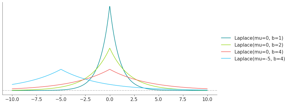
class preliz.distributions.logistic.Logistic(mu=None, s=None)[source]#

Logistic distribution.

The pdf of this distribution is

\[f(x \mid \mu, s) = \frac{ \exp ( - \frac{x - \mu}{s})}{s(1 + \exp ( - \frac{x - \mu}{s}))^2}\]

(Source code, png, hires.png, pdf)

Support	$x \in \mathbb{R}$
Mean	$\mu$
Variance	$\frac{s^2 \pi^2}{3}$

Parameters:

mu (float) – Mean.
s (float) – Scale (s > 0).

cdf(x)[source]#

Cumulative distribution function.

Parameters:: x (array_like) – Values on which to evaluate the cdf

entropy()[source]#: Entropy.

eti(mass=None, fmt='.2f')#

Equal-tailed interval containing mass.

Parameters:

mass (float) – Probability mass in the interval. Defaults to None,
used. (which results in the value of rcParams["stats.ci_prob"] being)
fmt (str) – fmt used to represent results using f-string fmt for floats. Default to “.2f” i.e. 2 digits after the decimal point. Use “none” for no format.

hdi(mass=None, fmt='.2f')#

Highest density interval containing mass.

Parameters:

mass (float) – Probability mass in the interval. Defaults to None,
used. (which results in the value of rcParams["stats.ci_prob"] being)
fmt (str) – fmt used to represent results using f-string fmt for floats. Default to “.2f” i.e. 2 digits after the decimal point. Use “none” for no format.

isf(x)#

Inverse survival function (inverse of sf).

Parameters:: x (array_like) – Values on which to evaluate the inverse of the sf

kurtosis()[source]#: Excess kurtosis.

lmoment1()[source]#: L-moment1 (mean).

lmoment2()[source]#: L-moment2 (l-scale).

lmoment3()[source]#: L-moment3 (l-skewness). This the ratio of L-moment3 to L-moment2.

lmoment4()[source]#: L-moment4 (l-kurtosis). This the ratio of L-moment4 to L-moment2.

lmoments(types='1234')#

Compute L-moments of the distribution.

Parameters:: types (str) – The type of moments to compute. Default is ‘1234’ where ‘1’ = L-moment1 (mean), ‘2’ = L-moment2 (l-scale), ‘3’ = L-moment3 (l-skewness), and ‘4’ = L-moment4 (l-kurtosis). To compute the standard deviation use ‘d’ Valid combinations are any subset of ‘1234’.

logcdf(x)#

Log cumulative distribution function.

Parameters:: x (array_like) – Values on which to evaluate the logcdf

logpdf(x)[source]#

Log probability density/mass function.

Parameters:: x (array_like) – Values on which to evaluate the logpdf

logsf(x)#

Log survival function log(1 - cdf).

Parameters:: x (array_like) – Values on which to evaluate the logsf

mean()[source]#: Mean.

median()[source]#: Median.

mode()[source]#: Mode.

moments(types='mvsk')#

Compute moments of the distribution.

It can also return the standard deviation

Parameters:: types (str) – The type of moments to compute. Default is ‘mvsk’ where ‘m’ = mean, ‘v’ = variance, ‘s’ = skewness, and ‘k’ = kurtosis. To compute the standard deviation use ‘d’ Valid combinations are any subset of ‘mvdsk’.

pdf(x)[source]#

Probability density/mass function.

Parameters:: x (array_like) – Values on which to evaluate the pdf

plot_cdf(moments=None, pointinterval=False, interval=None, levels=None, support='restricted', legend='legend', figsize=None, ax=None, **kwargs)#

Plot the cumulative distribution function.

Parameters:

moments (str) – Compute moments. Use any combination of the strings m, d, v, s or k for the mean (μ), standard deviation (σ), variance (σ²), skew (γ) or kurtosis (κ) respectively. Other strings will be ignored. Defaults to None.
pointinterval (bool) – Whether to include a plot of the quantiles. Defaults to False. If True the default is to plot the median and two interquantiles ranges.
interval (str) – Type of interval. Available options are highest density interval “hdi” (default), equal tailed interval “eti” or intervals defined by arbitrary “quantiles”. Defaults to the value in rcParams[“stats.ci_kind”].
levels (list) – Mass of the intervals. For hdi or eti the number of elements should be 2 or 1. For quantiles the number of elements should be 5, 3, 1 or 0 (in this last case nothing will be plotted).
support (str:) – If full use the finite end-points to set the limits of the plot. For unbounded end-points or if restricted use the 0.001 and 0.999 quantiles to set the limits.
legend (str) – Whether to include a string with the distribution and its parameter as a "legend" a "title" or not include them None.
figsize (tuple) – Size of the figure
ax (matplotlib axes)
kwargs (keyword arguments) – Additional keyword arguments passed to matplotlib plot function. For example, color, alpha, linewidth, etc.

plot_interactive(kind='pdf', xy_lim='both', pointinterval=True, interval=None, levels=None, figsize=None)#

Interactive exploration of distributions parameters.

Parameters:

kind (str:) – Type of plot. Available options are pdf, cdf and ppf.
xy_lim (str or tuple) – Set the limits of the x-axis and/or y-axis. Defaults to “both”, the limits of both axis are fixed. Use “auto” for automatic rescaling of x-axis and y-axis. Or set them manually by passing a tuple of 4 elements, the first two for x-axis, the last two for y-axis. The tuple can have None.
pointinterval (bool) – Whether to include a plot of the quantiles. Defaults to False. If True the default is to plot the median and two interquantiles ranges.
interval (str) – Type of interval. Available options are highest density interval “hdi” (default), equal tailed interval “eti” or intervals defined by arbitrary “quantiles”. Defaults to the value in rcParams[“stats.ci_kind”].
levels (list) – Mass of the intervals. For hdi or eti the number of elements should be 2 or 1. For quantiles the number of elements should be 5, 3, 1 or 0 (in this last case nothing will be plotted).
figsize (tuple) – Size of the figure

plot_isf(moments=None, pointinterval=False, interval=None, levels=None, legend='legend', figsize=None, ax=None, **kwargs)#

Plot the inverse survival function.

Parameters:

moments (str) – Compute moments. Use any combination of the strings m, d, v, s or k for the mean (μ), standard deviation (σ), variance (σ²), skew (γ) or kurtosis (κ) respectively. Other strings will be ignored. Defaults to None.
pointinterval (bool) – Whether to include a plot of the quantiles. Defaults to False. If True the default is to plot the median and two interquantiles ranges.
interval (str) – Type of interval. Available options are highest density interval “hdi” (default), equal tailed interval “eti” or intervals defined by arbitrary “quantiles”. Defaults to the value in rcParams[“stats.ci_kind”].
levels (list) – Mass of the intervals. For hdi or eti the number of elements should be 2 or 1. For quantiles the number of elements should be 5, 3, 1 or 0 (in this last case nothing will be plotted).
legend (str) – Whether to include a string with the distribution and its parameter as a "legend" a "title" or not include them None.
figsize (tuple) – Size of the figure
ax (matplotlib axes)

plot_pdf(moments=None, pointinterval=False, interval=None, levels=None, support='restricted', baseline=True, legend='legend', figsize=None, ax=None, **kwargs)#

Plot the pdf (continuous) or pmf (discrete).

Parameters:

moments (str) – Compute moments. Use any combination of the strings m, d, v, s or k for the mean (μ), standard deviation (σ), variance (σ²), skew (γ) or kurtosis (κ) respectively. Other strings will be ignored. Defaults to None.
pointinterval (bool) – Whether to include a plot of the quantiles. Defaults to False. If True the default is to plot the median and two interquantiles ranges.
interval (str) – Type of interval. Available options are highest density interval “hdi” (default), equal tailed interval “eti” or intervals defined by arbitrary “quantiles”. Defaults to the value in rcParams[“stats.ci_kind”].
levels (list) – Mass of the intervals. For hdi or eti the number of elements should be 2 or 1. For quantiles the number of elements should be 5, 3, 1 or 0 (in this last case nothing will be plotted).
support (str:) – If full use the finite end-points to set the limits of the plot. For unbounded end-points or if restricted use the 0.001 and 0.999 quantiles to set the limits.
baseline (bool) – Whether to include a horizontal line at y=0.
legend (str) – Whether to include a string with the distribution and its parameter as a "legend" a "title" or not include them None.
figsize (tuple) – Size of the figure
ax (matplotlib axes)
kwargs (keyword arguments) – Additional keyword arguments passed to matplotlib plot function. For example, color, alpha, linewidth, etc.

plot_ppf(moments=None, pointinterval=False, interval=None, levels=None, legend='legend', figsize=None, ax=None, **kwargs)#

Plot the quantile function.

Parameters:

moments (str) – Compute moments. Use any combination of the strings m, d, v, s or k for the mean (μ), standard deviation (σ), variance (σ²), skew (γ) or kurtosis (κ) respectively. Other strings will be ignored. Defaults to None.
pointinterval (bool) – Whether to include a plot of the quantiles. Defaults to False. If True the default is to plot the median and two interquantiles ranges.
interval (str) – Type of interval. Available options are highest density interval “hdi” (default), equal tailed interval “eti” or intervals defined by arbitrary “quantiles”. Defaults to the value in rcParams[“stats.ci_kind”].
levels (list) – Mass of the intervals. For hdi or eti the number of elements should be 2 or 1. For quantiles the number of elements should be 5, 3, 1 or 0 (in this last case nothing will be plotted).
legend (str) – Whether to include a string with the distribution and its parameter as a "legend" a "title" or not include them None.
figsize (tuple) – Size of the figure
ax (matplotlib axes)

plot_sf(moments=None, pointinterval=False, interval=None, levels=None, support='restricted', legend='legend', figsize=None, ax=None, **kwargs)#

Plot the survival distribution function (1 - CDF).

Parameters:

moments (str) – Compute moments. Use any combination of the strings m, d, v, s or k for the mean (μ), standard deviation (σ), variance (σ²), skew (γ) or kurtosis (κ) respectively. Other strings will be ignored. Defaults to None.
pointinterval (bool) – Whether to include a plot of the quantiles. Defaults to False. If True the default is to plot the median and two interquantiles ranges.
interval (str) – Type of interval. Available options are highest density interval “hdi” (default), equal tailed interval “eti” or intervals defined by arbitrary “quantiles”. Defaults to the value in rcParams[“stats.ci_kind”].
levels (list) – Mass of the intervals. For hdi or eti the number of elements should be 2 or 1. For quantiles the number of elements should be 5, 3, 1 or 0 (in this last case nothing will be plotted).
support (str:) – If full use the finite end-points to set the limits of the plot. For unbounded end-points or if restricted use the 0.001 and 0.999 quantiles to set the limits.
legend (str) – Whether to include a string with the distribution and its parameter as a "legend" a "title" or not include them None.
figsize (tuple) – Size of the figure
ax (matplotlib axes)
kwargs (keyword arguments) – Additional keyword arguments passed to matplotlib plot function. For example, color, alpha, linewidth, etc.

ppf(q)[source]#

Percent point function (inverse of cdf).

Parameters:: x (array_like) – Values on which to evaluate the inverse of the cdf

rvs(size=None, random_state=None)[source]#

Random sample.

Parameters:

size (int or tuple of ints, optional) – Defining number of random variates. Defaults to 1.
random_state ({None, int, numpy.random.Generator, numpy.random.RandomState}) – Defaults to None

sf(x)#

Survival function (1 - cdf).

Parameters:: x (array_like) – Values on which to evaluate the sf

skewness()[source]#: Skewness.

std()[source]#: Standard deviation.

summary(mass=None, interval=None, fmt='.2f')#

Namedtuple with the mean, median, sd, and lower and upper bounds.

Parameters:

mass (float) – Probability mass for the equal-tailed interval. Defaults to None,
used. (which results in the value of rcParams["stats.ci_prob"] being)
interval (str or list-like) – Type of interval. Available options are highest density interval “hdi”, equal tailed interval “eti” or arbitrary interval defined by a list-like object with a pair of values. Defaults to the value in rcParams[“stats.ci_kind”].
fmt (str) – fmt used to represent results using f-string fmt for floats. Default to “.2f” i.e. 2 digits after the decimal point.

to_bambi(**kwargs)#

Convert the PreliZ distribution to a Bambi Prior.

kwargsPyMC distributions properties: kwargs are used to specify properties such as shape or dims

Return type:: Bambi Prior

to_pymc(name=None, **kwargs)#

Convert the PreliZ distribution to a PyMC distribution.

namestr: Name of PyMC distribution. Needed if inside Model context
kwargsPyMC distributions properties: kwargs are used to specify properties such as shape or dims

Return type:: PyMC distribution

var()[source]#: Variance.

xvals(support, n_points=None)#

Provide x values in the support of the distribution.

This is useful for example when plotting.

Parameters:

support (str) – Available options are “full” or “restricted”. If “full” the values will cover the entire support of the distribution if the boundary is finite, or the quantiles 0.0001 or 0.9999, if infinite. If “restricted” the values will cover the quantile 0.0001 to 0.9999.
n_points (int) – Number of values to return. Defaults to 1000 for continuous distributions and 200 for discrete ones. For discrete distributions the returned values may be fewer than n_points if the actual number of discrete values in the support of the distribution is smaller than n_points.

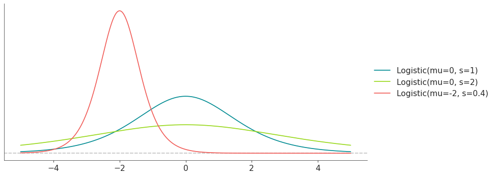
class preliz.distributions.loglogistic.LogLogistic(alpha=None, beta=None)[source]#

Log-Logistic distribution.

Also known as the Fisk distribution is a continuous non-negative distribution used in survival analysis as a parametric model for events whose rate increases initially and decreases later

The pdf of this distribution is

\[f(x\mid \alpha, \beta) = \frac{ (\beta/\alpha)(x/\alpha)^{\beta-1}} {\left( 1+(x/\alpha)^{\beta} \right)^2}\]

(Source code, png, hires.png, pdf)

Support	$x \in [0, \infty)$
Mean	${\alpha\,\pi/\beta \over \sin(\pi/\beta)}$
Variance	$\alpha^2 \left(2b / \sin 2b -b^2 / \sin^2 b \right), \quad \beta>2$

Parameters:

alpha (float) – Scale parameter. (alpha > 0))
beta (float) – Shape parameter. (beta > 0)).

cdf(x)[source]#

Cumulative distribution function.

Parameters:: x (array_like) – Values on which to evaluate the cdf

entropy()[source]#: Entropy.

eti(mass=None, fmt='.2f')#

Equal-tailed interval containing mass.

Parameters:

mass (float) – Probability mass in the interval. Defaults to None,
used. (which results in the value of rcParams["stats.ci_prob"] being)
fmt (str) – fmt used to represent results using f-string fmt for floats. Default to “.2f” i.e. 2 digits after the decimal point. Use “none” for no format.

hdi(mass=None, fmt='.2f')#

Highest density interval containing mass.

Parameters:

mass (float) – Probability mass in the interval. Defaults to None,
used. (which results in the value of rcParams["stats.ci_prob"] being)
fmt (str) – fmt used to represent results using f-string fmt for floats. Default to “.2f” i.e. 2 digits after the decimal point. Use “none” for no format.

isf(x)#

Inverse survival function (inverse of sf).

Parameters:: x (array_like) – Values on which to evaluate the inverse of the sf

kurtosis()[source]#: Excess kurtosis.

lmoment1()[source]#: L-moment1 (mean).

lmoment2()[source]#: L-moment2 (l-scale).

lmoment3()[source]#: L-moment3 (l-skewness). This the ratio of L-moment3 to L-moment2.

lmoment4()[source]#: L-moment4 (l-kurtosis). This the ratio of L-moment4 to L-moment2.

lmoments(types='1234')#

Compute L-moments of the distribution.

Parameters:: types (str) – The type of moments to compute. Default is ‘1234’ where ‘1’ = L-moment1 (mean), ‘2’ = L-moment2 (l-scale), ‘3’ = L-moment3 (l-skewness), and ‘4’ = L-moment4 (l-kurtosis). To compute the standard deviation use ‘d’ Valid combinations are any subset of ‘1234’.

logcdf(x)#

Log cumulative distribution function.

Parameters:: x (array_like) – Values on which to evaluate the logcdf

logpdf(x)[source]#

Log probability density/mass function.

Parameters:: x (array_like) – Values on which to evaluate the logpdf

logsf(x)#

Log survival function log(1 - cdf).

Parameters:: x (array_like) – Values on which to evaluate the logsf

mean()[source]#: Mean.

median()[source]#: Median.

mode()[source]#: Mode.

moments(types='mvsk')#

Compute moments of the distribution.

It can also return the standard deviation

Parameters:: types (str) – The type of moments to compute. Default is ‘mvsk’ where ‘m’ = mean, ‘v’ = variance, ‘s’ = skewness, and ‘k’ = kurtosis. To compute the standard deviation use ‘d’ Valid combinations are any subset of ‘mvdsk’.

pdf(x)[source]#

Probability density/mass function.

Parameters:: x (array_like) – Values on which to evaluate the pdf

plot_cdf(moments=None, pointinterval=False, interval=None, levels=None, support='restricted', legend='legend', figsize=None, ax=None, **kwargs)#

Plot the cumulative distribution function.

Parameters:

moments (str) – Compute moments. Use any combination of the strings m, d, v, s or k for the mean (μ), standard deviation (σ), variance (σ²), skew (γ) or kurtosis (κ) respectively. Other strings will be ignored. Defaults to None.
pointinterval (bool) – Whether to include a plot of the quantiles. Defaults to False. If True the default is to plot the median and two interquantiles ranges.
interval (str) – Type of interval. Available options are highest density interval “hdi” (default), equal tailed interval “eti” or intervals defined by arbitrary “quantiles”. Defaults to the value in rcParams[“stats.ci_kind”].
levels (list) – Mass of the intervals. For hdi or eti the number of elements should be 2 or 1. For quantiles the number of elements should be 5, 3, 1 or 0 (in this last case nothing will be plotted).
support (str:) – If full use the finite end-points to set the limits of the plot. For unbounded end-points or if restricted use the 0.001 and 0.999 quantiles to set the limits.
legend (str) – Whether to include a string with the distribution and its parameter as a "legend" a "title" or not include them None.
figsize (tuple) – Size of the figure
ax (matplotlib axes)
kwargs (keyword arguments) – Additional keyword arguments passed to matplotlib plot function. For example, color, alpha, linewidth, etc.

plot_interactive(kind='pdf', xy_lim='both', pointinterval=True, interval=None, levels=None, figsize=None)#

Interactive exploration of distributions parameters.

Parameters:

kind (str:) – Type of plot. Available options are pdf, cdf and ppf.
xy_lim (str or tuple) – Set the limits of the x-axis and/or y-axis. Defaults to “both”, the limits of both axis are fixed. Use “auto” for automatic rescaling of x-axis and y-axis. Or set them manually by passing a tuple of 4 elements, the first two for x-axis, the last two for y-axis. The tuple can have None.
pointinterval (bool) – Whether to include a plot of the quantiles. Defaults to False. If True the default is to plot the median and two interquantiles ranges.
interval (str) – Type of interval. Available options are highest density interval “hdi” (default), equal tailed interval “eti” or intervals defined by arbitrary “quantiles”. Defaults to the value in rcParams[“stats.ci_kind”].
levels (list) – Mass of the intervals. For hdi or eti the number of elements should be 2 or 1. For quantiles the number of elements should be 5, 3, 1 or 0 (in this last case nothing will be plotted).
figsize (tuple) – Size of the figure

plot_isf(moments=None, pointinterval=False, interval=None, levels=None, legend='legend', figsize=None, ax=None, **kwargs)#

Plot the inverse survival function.

Parameters:

moments (str) – Compute moments. Use any combination of the strings m, d, v, s or k for the mean (μ), standard deviation (σ), variance (σ²), skew (γ) or kurtosis (κ) respectively. Other strings will be ignored. Defaults to None.
pointinterval (bool) – Whether to include a plot of the quantiles. Defaults to False. If True the default is to plot the median and two interquantiles ranges.
interval (str) – Type of interval. Available options are highest density interval “hdi” (default), equal tailed interval “eti” or intervals defined by arbitrary “quantiles”. Defaults to the value in rcParams[“stats.ci_kind”].
levels (list) – Mass of the intervals. For hdi or eti the number of elements should be 2 or 1. For quantiles the number of elements should be 5, 3, 1 or 0 (in this last case nothing will be plotted).
legend (str) – Whether to include a string with the distribution and its parameter as a "legend" a "title" or not include them None.
figsize (tuple) – Size of the figure
ax (matplotlib axes)

plot_pdf(moments=None, pointinterval=False, interval=None, levels=None, support='restricted', baseline=True, legend='legend', figsize=None, ax=None, **kwargs)#

Plot the pdf (continuous) or pmf (discrete).

Parameters:

moments (str) – Compute moments. Use any combination of the strings m, d, v, s or k for the mean (μ), standard deviation (σ), variance (σ²), skew (γ) or kurtosis (κ) respectively. Other strings will be ignored. Defaults to None.
pointinterval (bool) – Whether to include a plot of the quantiles. Defaults to False. If True the default is to plot the median and two interquantiles ranges.
interval (str) – Type of interval. Available options are highest density interval “hdi” (default), equal tailed interval “eti” or intervals defined by arbitrary “quantiles”. Defaults to the value in rcParams[“stats.ci_kind”].
levels (list) – Mass of the intervals. For hdi or eti the number of elements should be 2 or 1. For quantiles the number of elements should be 5, 3, 1 or 0 (in this last case nothing will be plotted).
support (str:) – If full use the finite end-points to set the limits of the plot. For unbounded end-points or if restricted use the 0.001 and 0.999 quantiles to set the limits.
baseline (bool) – Whether to include a horizontal line at y=0.
legend (str) – Whether to include a string with the distribution and its parameter as a "legend" a "title" or not include them None.
figsize (tuple) – Size of the figure
ax (matplotlib axes)
kwargs (keyword arguments) – Additional keyword arguments passed to matplotlib plot function. For example, color, alpha, linewidth, etc.

plot_ppf(moments=None, pointinterval=False, interval=None, levels=None, legend='legend', figsize=None, ax=None, **kwargs)#

Plot the quantile function.

Parameters:

moments (str) – Compute moments. Use any combination of the strings m, d, v, s or k for the mean (μ), standard deviation (σ), variance (σ²), skew (γ) or kurtosis (κ) respectively. Other strings will be ignored. Defaults to None.
pointinterval (bool) – Whether to include a plot of the quantiles. Defaults to False. If True the default is to plot the median and two interquantiles ranges.
interval (str) – Type of interval. Available options are highest density interval “hdi” (default), equal tailed interval “eti” or intervals defined by arbitrary “quantiles”. Defaults to the value in rcParams[“stats.ci_kind”].
levels (list) – Mass of the intervals. For hdi or eti the number of elements should be 2 or 1. For quantiles the number of elements should be 5, 3, 1 or 0 (in this last case nothing will be plotted).
legend (str) – Whether to include a string with the distribution and its parameter as a "legend" a "title" or not include them None.
figsize (tuple) – Size of the figure
ax (matplotlib axes)

plot_sf(moments=None, pointinterval=False, interval=None, levels=None, support='restricted', legend='legend', figsize=None, ax=None, **kwargs)#

Plot the survival distribution function (1 - CDF).

Parameters:

moments (str) – Compute moments. Use any combination of the strings m, d, v, s or k for the mean (μ), standard deviation (σ), variance (σ²), skew (γ) or kurtosis (κ) respectively. Other strings will be ignored. Defaults to None.
pointinterval (bool) – Whether to include a plot of the quantiles. Defaults to False. If True the default is to plot the median and two interquantiles ranges.
interval (str) – Type of interval. Available options are highest density interval “hdi” (default), equal tailed interval “eti” or intervals defined by arbitrary “quantiles”. Defaults to the value in rcParams[“stats.ci_kind”].
levels (list) – Mass of the intervals. For hdi or eti the number of elements should be 2 or 1. For quantiles the number of elements should be 5, 3, 1 or 0 (in this last case nothing will be plotted).
support (str:) – If full use the finite end-points to set the limits of the plot. For unbounded end-points or if restricted use the 0.001 and 0.999 quantiles to set the limits.
legend (str) – Whether to include a string with the distribution and its parameter as a "legend" a "title" or not include them None.
figsize (tuple) – Size of the figure
ax (matplotlib axes)
kwargs (keyword arguments) – Additional keyword arguments passed to matplotlib plot function. For example, color, alpha, linewidth, etc.

ppf(q)[source]#

Percent point function (inverse of cdf).

Parameters:: x (array_like) – Values on which to evaluate the inverse of the cdf

rvs(size=None, random_state=None)[source]#

Random sample.

Parameters:

size (int or tuple of ints, optional) – Defining number of random variates. Defaults to 1.
random_state ({None, int, numpy.random.Generator, numpy.random.RandomState}) – Defaults to None

sf(x)#

Survival function (1 - cdf).

Parameters:: x (array_like) – Values on which to evaluate the sf

skewness()[source]#: Skewness.

std()[source]#: Standard deviation.

summary(mass=None, interval=None, fmt='.2f')#

Namedtuple with the mean, median, sd, and lower and upper bounds.

Parameters:

mass (float) – Probability mass for the equal-tailed interval. Defaults to None,
used. (which results in the value of rcParams["stats.ci_prob"] being)
interval (str or list-like) – Type of interval. Available options are highest density interval “hdi”, equal tailed interval “eti” or arbitrary interval defined by a list-like object with a pair of values. Defaults to the value in rcParams[“stats.ci_kind”].
fmt (str) – fmt used to represent results using f-string fmt for floats. Default to “.2f” i.e. 2 digits after the decimal point.

to_bambi(**kwargs)#

Convert the PreliZ distribution to a Bambi Prior.

kwargsPyMC distributions properties: kwargs are used to specify properties such as shape or dims

Return type:: Bambi Prior

to_pymc(name=None, **kwargs)#

Convert the PreliZ distribution to a PyMC distribution.

namestr: Name of PyMC distribution. Needed if inside Model context
kwargsPyMC distributions properties: kwargs are used to specify properties such as shape or dims

Return type:: PyMC distribution

var()[source]#: Variance.

xvals(support, n_points=None)#

Provide x values in the support of the distribution.

This is useful for example when plotting.

Parameters:

support (str) – Available options are “full” or “restricted”. If “full” the values will cover the entire support of the distribution if the boundary is finite, or the quantiles 0.0001 or 0.9999, if infinite. If “restricted” the values will cover the quantile 0.0001 to 0.9999.
n_points (int) – Number of values to return. Defaults to 1000 for continuous distributions and 200 for discrete ones. For discrete distributions the returned values may be fewer than n_points if the actual number of discrete values in the support of the distribution is smaller than n_points.

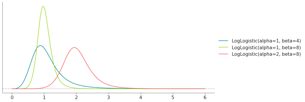
class preliz.distributions.logitnormal.LogitNormal(mu=None, sigma=None, tau=None)[source]#

Logit-Normal distribution.

The pdf of this distribution is

\[f(x \mid \mu, \tau) = \frac{1}{x(1-x)} \sqrt{\frac{\tau}{2\pi}} \exp\left\{ -\frac{\tau}{2} (logit(x)-\mu)^2 \right\}\]

(Source code, png, hires.png, pdf)

Support	$x \in (0, 1)$
Mean	no analytical solution
Variance	no analytical solution

Parameters:

mu (float) – Location parameter.
sigma (float) – Scale parameter (sigma > 0).
tau (float) – Scale parameter (tau > 0).

cdf(x)[source]#

Cumulative distribution function.

Parameters:: x (array_like) – Values on which to evaluate the cdf

entropy()[source]#: Entropy.

eti(mass=None, fmt='.2f')#

Equal-tailed interval containing mass.

Parameters:

mass (float) – Probability mass in the interval. Defaults to None,
used. (which results in the value of rcParams["stats.ci_prob"] being)
fmt (str) – fmt used to represent results using f-string fmt for floats. Default to “.2f” i.e. 2 digits after the decimal point. Use “none” for no format.

hdi(mass=None, fmt='.2f')#

Highest density interval containing mass.

Parameters:

mass (float) – Probability mass in the interval. Defaults to None,
used. (which results in the value of rcParams["stats.ci_prob"] being)
fmt (str) – fmt used to represent results using f-string fmt for floats. Default to “.2f” i.e. 2 digits after the decimal point. Use “none” for no format.

isf(x)#

Inverse survival function (inverse of sf).

Parameters:: x (array_like) – Values on which to evaluate the inverse of the sf

kurtosis()[source]#: Excess kurtosis.

lmoment1()[source]#: L-moment1 (mean).

lmoment2()[source]#: L-moment2 (l-scale).

lmoment3()[source]#: L-moment3 (l-skewness). This the ratio of L-moment3 to L-moment2.

lmoment4()[source]#: L-moment4 (l-kurtosis). This the ratio of L-moment4 to L-moment2.

lmoments(types='1234')#

Compute L-moments of the distribution.

Parameters:: types (str) – The type of moments to compute. Default is ‘1234’ where ‘1’ = L-moment1 (mean), ‘2’ = L-moment2 (l-scale), ‘3’ = L-moment3 (l-skewness), and ‘4’ = L-moment4 (l-kurtosis). To compute the standard deviation use ‘d’ Valid combinations are any subset of ‘1234’.

logcdf(x)#

Log cumulative distribution function.

Parameters:: x (array_like) – Values on which to evaluate the logcdf

logpdf(x)[source]#

Log probability density/mass function.

Parameters:: x (array_like) – Values on which to evaluate the logpdf

logsf(x)#

Log survival function log(1 - cdf).

Parameters:: x (array_like) – Values on which to evaluate the logsf

mean()[source]#: Mean.

median()[source]#: Median.

mode()[source]#: Mode.

moments(types='mvsk')#

Compute moments of the distribution.

It can also return the standard deviation

Parameters:: types (str) – The type of moments to compute. Default is ‘mvsk’ where ‘m’ = mean, ‘v’ = variance, ‘s’ = skewness, and ‘k’ = kurtosis. To compute the standard deviation use ‘d’ Valid combinations are any subset of ‘mvdsk’.

pdf(x)[source]#

Probability density/mass function.

Parameters:: x (array_like) – Values on which to evaluate the pdf

plot_cdf(moments=None, pointinterval=False, interval=None, levels=None, support='restricted', legend='legend', figsize=None, ax=None, **kwargs)#

Plot the cumulative distribution function.

Parameters:

moments (str) – Compute moments. Use any combination of the strings m, d, v, s or k for the mean (μ), standard deviation (σ), variance (σ²), skew (γ) or kurtosis (κ) respectively. Other strings will be ignored. Defaults to None.
pointinterval (bool) – Whether to include a plot of the quantiles. Defaults to False. If True the default is to plot the median and two interquantiles ranges.
interval (str) – Type of interval. Available options are highest density interval “hdi” (default), equal tailed interval “eti” or intervals defined by arbitrary “quantiles”. Defaults to the value in rcParams[“stats.ci_kind”].
levels (list) – Mass of the intervals. For hdi or eti the number of elements should be 2 or 1. For quantiles the number of elements should be 5, 3, 1 or 0 (in this last case nothing will be plotted).
support (str:) – If full use the finite end-points to set the limits of the plot. For unbounded end-points or if restricted use the 0.001 and 0.999 quantiles to set the limits.
legend (str) – Whether to include a string with the distribution and its parameter as a "legend" a "title" or not include them None.
figsize (tuple) – Size of the figure
ax (matplotlib axes)
kwargs (keyword arguments) – Additional keyword arguments passed to matplotlib plot function. For example, color, alpha, linewidth, etc.

plot_interactive(kind='pdf', xy_lim='both', pointinterval=True, interval=None, levels=None, figsize=None)#

Interactive exploration of distributions parameters.

Parameters:

kind (str:) – Type of plot. Available options are pdf, cdf and ppf.
xy_lim (str or tuple) – Set the limits of the x-axis and/or y-axis. Defaults to “both”, the limits of both axis are fixed. Use “auto” for automatic rescaling of x-axis and y-axis. Or set them manually by passing a tuple of 4 elements, the first two for x-axis, the last two for y-axis. The tuple can have None.
pointinterval (bool) – Whether to include a plot of the quantiles. Defaults to False. If True the default is to plot the median and two interquantiles ranges.
interval (str) – Type of interval. Available options are highest density interval “hdi” (default), equal tailed interval “eti” or intervals defined by arbitrary “quantiles”. Defaults to the value in rcParams[“stats.ci_kind”].
levels (list) – Mass of the intervals. For hdi or eti the number of elements should be 2 or 1. For quantiles the number of elements should be 5, 3, 1 or 0 (in this last case nothing will be plotted).
figsize (tuple) – Size of the figure

plot_isf(moments=None, pointinterval=False, interval=None, levels=None, legend='legend', figsize=None, ax=None, **kwargs)#

Plot the inverse survival function.

Parameters:

moments (str) – Compute moments. Use any combination of the strings m, d, v, s or k for the mean (μ), standard deviation (σ), variance (σ²), skew (γ) or kurtosis (κ) respectively. Other strings will be ignored. Defaults to None.
pointinterval (bool) – Whether to include a plot of the quantiles. Defaults to False. If True the default is to plot the median and two interquantiles ranges.
interval (str) – Type of interval. Available options are highest density interval “hdi” (default), equal tailed interval “eti” or intervals defined by arbitrary “quantiles”. Defaults to the value in rcParams[“stats.ci_kind”].
levels (list) – Mass of the intervals. For hdi or eti the number of elements should be 2 or 1. For quantiles the number of elements should be 5, 3, 1 or 0 (in this last case nothing will be plotted).
legend (str) – Whether to include a string with the distribution and its parameter as a "legend" a "title" or not include them None.
figsize (tuple) – Size of the figure
ax (matplotlib axes)

plot_pdf(moments=None, pointinterval=False, interval=None, levels=None, support='restricted', baseline=True, legend='legend', figsize=None, ax=None, **kwargs)#

Plot the pdf (continuous) or pmf (discrete).

Parameters:

moments (str) – Compute moments. Use any combination of the strings m, d, v, s or k for the mean (μ), standard deviation (σ), variance (σ²), skew (γ) or kurtosis (κ) respectively. Other strings will be ignored. Defaults to None.
pointinterval (bool) – Whether to include a plot of the quantiles. Defaults to False. If True the default is to plot the median and two interquantiles ranges.
interval (str) – Type of interval. Available options are highest density interval “hdi” (default), equal tailed interval “eti” or intervals defined by arbitrary “quantiles”. Defaults to the value in rcParams[“stats.ci_kind”].
levels (list) – Mass of the intervals. For hdi or eti the number of elements should be 2 or 1. For quantiles the number of elements should be 5, 3, 1 or 0 (in this last case nothing will be plotted).
support (str:) – If full use the finite end-points to set the limits of the plot. For unbounded end-points or if restricted use the 0.001 and 0.999 quantiles to set the limits.
baseline (bool) – Whether to include a horizontal line at y=0.
legend (str) – Whether to include a string with the distribution and its parameter as a "legend" a "title" or not include them None.
figsize (tuple) – Size of the figure
ax (matplotlib axes)
kwargs (keyword arguments) – Additional keyword arguments passed to matplotlib plot function. For example, color, alpha, linewidth, etc.

plot_ppf(moments=None, pointinterval=False, interval=None, levels=None, legend='legend', figsize=None, ax=None, **kwargs)#

Plot the quantile function.

Parameters:

moments (str) – Compute moments. Use any combination of the strings m, d, v, s or k for the mean (μ), standard deviation (σ), variance (σ²), skew (γ) or kurtosis (κ) respectively. Other strings will be ignored. Defaults to None.
pointinterval (bool) – Whether to include a plot of the quantiles. Defaults to False. If True the default is to plot the median and two interquantiles ranges.
interval (str) – Type of interval. Available options are highest density interval “hdi” (default), equal tailed interval “eti” or intervals defined by arbitrary “quantiles”. Defaults to the value in rcParams[“stats.ci_kind”].
levels (list) – Mass of the intervals. For hdi or eti the number of elements should be 2 or 1. For quantiles the number of elements should be 5, 3, 1 or 0 (in this last case nothing will be plotted).
legend (str) – Whether to include a string with the distribution and its parameter as a "legend" a "title" or not include them None.
figsize (tuple) – Size of the figure
ax (matplotlib axes)

plot_sf(moments=None, pointinterval=False, interval=None, levels=None, support='restricted', legend='legend', figsize=None, ax=None, **kwargs)#

Plot the survival distribution function (1 - CDF).

Parameters:

moments (str) – Compute moments. Use any combination of the strings m, d, v, s or k for the mean (μ), standard deviation (σ), variance (σ²), skew (γ) or kurtosis (κ) respectively. Other strings will be ignored. Defaults to None.
pointinterval (bool) – Whether to include a plot of the quantiles. Defaults to False. If True the default is to plot the median and two interquantiles ranges.
interval (str) – Type of interval. Available options are highest density interval “hdi” (default), equal tailed interval “eti” or intervals defined by arbitrary “quantiles”. Defaults to the value in rcParams[“stats.ci_kind”].
levels (list) – Mass of the intervals. For hdi or eti the number of elements should be 2 or 1. For quantiles the number of elements should be 5, 3, 1 or 0 (in this last case nothing will be plotted).
support (str:) – If full use the finite end-points to set the limits of the plot. For unbounded end-points or if restricted use the 0.001 and 0.999 quantiles to set the limits.
legend (str) – Whether to include a string with the distribution and its parameter as a "legend" a "title" or not include them None.
figsize (tuple) – Size of the figure
ax (matplotlib axes)
kwargs (keyword arguments) – Additional keyword arguments passed to matplotlib plot function. For example, color, alpha, linewidth, etc.

ppf(q)[source]#

Percent point function (inverse of cdf).

Parameters:: x (array_like) – Values on which to evaluate the inverse of the cdf

rvs(size=None, random_state=None)[source]#

Random sample.

Parameters:

size (int or tuple of ints, optional) – Defining number of random variates. Defaults to 1.
random_state ({None, int, numpy.random.Generator, numpy.random.RandomState}) – Defaults to None

sf(x)#

Survival function (1 - cdf).

Parameters:: x (array_like) – Values on which to evaluate the sf

skewness()[source]#: Skewness.

std()[source]#: Standard deviation.

summary(mass=None, interval=None, fmt='.2f')#

Namedtuple with the mean, median, sd, and lower and upper bounds.

Parameters:

mass (float) – Probability mass for the equal-tailed interval. Defaults to None,
used. (which results in the value of rcParams["stats.ci_prob"] being)
interval (str or list-like) – Type of interval. Available options are highest density interval “hdi”, equal tailed interval “eti” or arbitrary interval defined by a list-like object with a pair of values. Defaults to the value in rcParams[“stats.ci_kind”].
fmt (str) – fmt used to represent results using f-string fmt for floats. Default to “.2f” i.e. 2 digits after the decimal point.

to_bambi(**kwargs)#

Convert the PreliZ distribution to a Bambi Prior.

kwargsPyMC distributions properties: kwargs are used to specify properties such as shape or dims

Return type:: Bambi Prior

to_pymc(name=None, **kwargs)#

Convert the PreliZ distribution to a PyMC distribution.

namestr: Name of PyMC distribution. Needed if inside Model context
kwargsPyMC distributions properties: kwargs are used to specify properties such as shape or dims

Return type:: PyMC distribution

var()[source]#: Variance.

xvals(support, n_points=None)#

Provide x values in the support of the distribution.

This is useful for example when plotting.

Parameters:

support (str) – Available options are “full” or “restricted”. If “full” the values will cover the entire support of the distribution if the boundary is finite, or the quantiles 0.0001 or 0.9999, if infinite. If “restricted” the values will cover the quantile 0.0001 to 0.9999.
n_points (int) – Number of values to return. Defaults to 1000 for continuous distributions and 200 for discrete ones. For discrete distributions the returned values may be fewer than n_points if the actual number of discrete values in the support of the distribution is smaller than n_points.

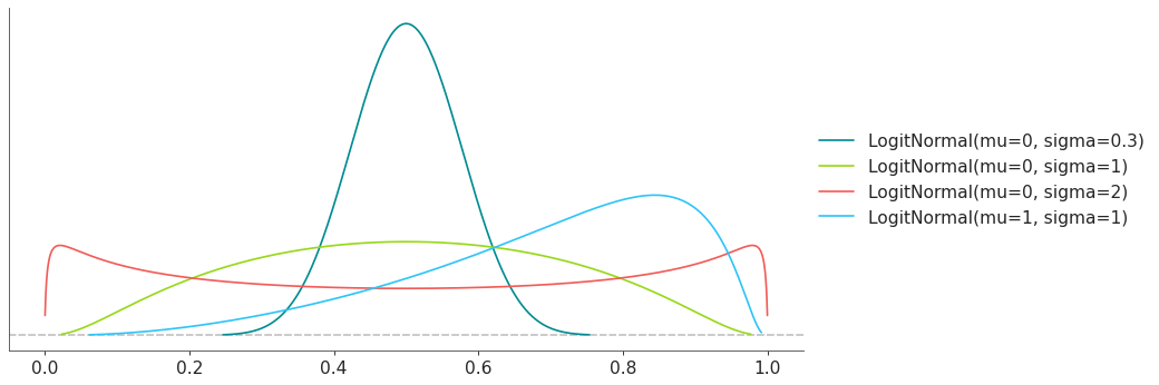
class preliz.distributions.lognormal.LogNormal(mu=None, sigma=None)[source]#

Log-normal distribution.

Distribution of any random variable whose logarithm is normally distributed. A variable might be modeled as log-normal if it can be thought of as the multiplicative product of many small independent factors.

The pdf of this distribution is

\[f(x \mid \mu, \sigma) = \frac{1}{x \sigma \sqrt{2\pi}} \exp\left\{ -\frac{(\ln(x)-\mu)^2}{2\sigma^2} \right\}\]

(Source code, png, hires.png, pdf)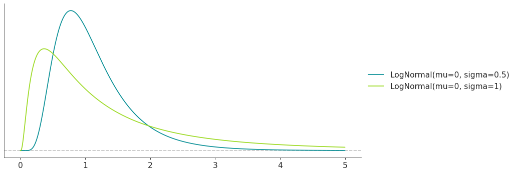

Support	$x \in [0, \infty)$
Mean	$\exp\left(\mu+\frac{\sigma^2}{2}\right)$
Variance	$[\exp(\sigma^2)-1] \exp(2\mu+\sigma^2)$

Parameters:

mu (float) – Location parameter.
sigma (float) – Standard deviation. (sigma > 0)).

cdf(x)[source]#

Cumulative distribution function.

Parameters:: x (array_like) – Values on which to evaluate the cdf

entropy()[source]#: Entropy.

eti(mass=None, fmt='.2f')#

Equal-tailed interval containing mass.

Parameters:

mass (float) – Probability mass in the interval. Defaults to None,
used. (which results in the value of rcParams["stats.ci_prob"] being)
fmt (str) – fmt used to represent results using f-string fmt for floats. Default to “.2f” i.e. 2 digits after the decimal point. Use “none” for no format.

hdi(mass=None, fmt='.2f')#

Highest density interval containing mass.

Parameters:

mass (float) – Probability mass in the interval. Defaults to None,
used. (which results in the value of rcParams["stats.ci_prob"] being)
fmt (str) – fmt used to represent results using f-string fmt for floats. Default to “.2f” i.e. 2 digits after the decimal point. Use “none” for no format.

isf(x)#

Inverse survival function (inverse of sf).

Parameters:: x (array_like) – Values on which to evaluate the inverse of the sf

kurtosis()[source]#: Excess kurtosis.

lmoment1()[source]#: L-moment1 (mean).

lmoment2()[source]#: L-moment2 (l-scale).

lmoment3()[source]#: L-moment3 (l-skewness). This the ratio of L-moment3 to L-moment2.

lmoment4()[source]#: L-moment4 (l-kurtosis). This the ratio of L-moment4 to L-moment2.

lmoments(types='1234')#

Compute L-moments of the distribution.

Parameters:: types (str) – The type of moments to compute. Default is ‘1234’ where ‘1’ = L-moment1 (mean), ‘2’ = L-moment2 (l-scale), ‘3’ = L-moment3 (l-skewness), and ‘4’ = L-moment4 (l-kurtosis). To compute the standard deviation use ‘d’ Valid combinations are any subset of ‘1234’.

logcdf(x)#

Log cumulative distribution function.

Parameters:: x (array_like) – Values on which to evaluate the logcdf

logpdf(x)[source]#

Log probability density/mass function.

Parameters:: x (array_like) – Values on which to evaluate the logpdf

logsf(x)#

Log survival function log(1 - cdf).

Parameters:: x (array_like) – Values on which to evaluate the logsf

mean()[source]#: Mean.

median()[source]#: Median.

mode()[source]#: Mode.

moments(types='mvsk')#

Compute moments of the distribution.

It can also return the standard deviation

Parameters:: types (str) – The type of moments to compute. Default is ‘mvsk’ where ‘m’ = mean, ‘v’ = variance, ‘s’ = skewness, and ‘k’ = kurtosis. To compute the standard deviation use ‘d’ Valid combinations are any subset of ‘mvdsk’.

pdf(x)[source]#

Probability density/mass function.

Parameters:: x (array_like) – Values on which to evaluate the pdf

plot_cdf(moments=None, pointinterval=False, interval=None, levels=None, support='restricted', legend='legend', figsize=None, ax=None, **kwargs)#

Plot the cumulative distribution function.

Parameters:

moments (str) – Compute moments. Use any combination of the strings m, d, v, s or k for the mean (μ), standard deviation (σ), variance (σ²), skew (γ) or kurtosis (κ) respectively. Other strings will be ignored. Defaults to None.
pointinterval (bool) – Whether to include a plot of the quantiles. Defaults to False. If True the default is to plot the median and two interquantiles ranges.
interval (str) – Type of interval. Available options are highest density interval “hdi” (default), equal tailed interval “eti” or intervals defined by arbitrary “quantiles”. Defaults to the value in rcParams[“stats.ci_kind”].
levels (list) – Mass of the intervals. For hdi or eti the number of elements should be 2 or 1. For quantiles the number of elements should be 5, 3, 1 or 0 (in this last case nothing will be plotted).
support (str:) – If full use the finite end-points to set the limits of the plot. For unbounded end-points or if restricted use the 0.001 and 0.999 quantiles to set the limits.
legend (str) – Whether to include a string with the distribution and its parameter as a "legend" a "title" or not include them None.
figsize (tuple) – Size of the figure
ax (matplotlib axes)
kwargs (keyword arguments) – Additional keyword arguments passed to matplotlib plot function. For example, color, alpha, linewidth, etc.

plot_interactive(kind='pdf', xy_lim='both', pointinterval=True, interval=None, levels=None, figsize=None)#

Interactive exploration of distributions parameters.

Parameters:

kind (str:) – Type of plot. Available options are pdf, cdf and ppf.
xy_lim (str or tuple) – Set the limits of the x-axis and/or y-axis. Defaults to “both”, the limits of both axis are fixed. Use “auto” for automatic rescaling of x-axis and y-axis. Or set them manually by passing a tuple of 4 elements, the first two for x-axis, the last two for y-axis. The tuple can have None.
pointinterval (bool) – Whether to include a plot of the quantiles. Defaults to False. If True the default is to plot the median and two interquantiles ranges.
interval (str) – Type of interval. Available options are highest density interval “hdi” (default), equal tailed interval “eti” or intervals defined by arbitrary “quantiles”. Defaults to the value in rcParams[“stats.ci_kind”].
levels (list) – Mass of the intervals. For hdi or eti the number of elements should be 2 or 1. For quantiles the number of elements should be 5, 3, 1 or 0 (in this last case nothing will be plotted).
figsize (tuple) – Size of the figure

plot_isf(moments=None, pointinterval=False, interval=None, levels=None, legend='legend', figsize=None, ax=None, **kwargs)#

Plot the inverse survival function.

Parameters:

moments (str) – Compute moments. Use any combination of the strings m, d, v, s or k for the mean (μ), standard deviation (σ), variance (σ²), skew (γ) or kurtosis (κ) respectively. Other strings will be ignored. Defaults to None.
pointinterval (bool) – Whether to include a plot of the quantiles. Defaults to False. If True the default is to plot the median and two interquantiles ranges.
interval (str) – Type of interval. Available options are highest density interval “hdi” (default), equal tailed interval “eti” or intervals defined by arbitrary “quantiles”. Defaults to the value in rcParams[“stats.ci_kind”].
levels (list) – Mass of the intervals. For hdi or eti the number of elements should be 2 or 1. For quantiles the number of elements should be 5, 3, 1 or 0 (in this last case nothing will be plotted).
legend (str) – Whether to include a string with the distribution and its parameter as a "legend" a "title" or not include them None.
figsize (tuple) – Size of the figure
ax (matplotlib axes)

plot_pdf(moments=None, pointinterval=False, interval=None, levels=None, support='restricted', baseline=True, legend='legend', figsize=None, ax=None, **kwargs)#

Plot the pdf (continuous) or pmf (discrete).

Parameters:

moments (str) – Compute moments. Use any combination of the strings m, d, v, s or k for the mean (μ), standard deviation (σ), variance (σ²), skew (γ) or kurtosis (κ) respectively. Other strings will be ignored. Defaults to None.
pointinterval (bool) – Whether to include a plot of the quantiles. Defaults to False. If True the default is to plot the median and two interquantiles ranges.
interval (str) – Type of interval. Available options are highest density interval “hdi” (default), equal tailed interval “eti” or intervals defined by arbitrary “quantiles”. Defaults to the value in rcParams[“stats.ci_kind”].
levels (list) – Mass of the intervals. For hdi or eti the number of elements should be 2 or 1. For quantiles the number of elements should be 5, 3, 1 or 0 (in this last case nothing will be plotted).
support (str:) – If full use the finite end-points to set the limits of the plot. For unbounded end-points or if restricted use the 0.001 and 0.999 quantiles to set the limits.
baseline (bool) – Whether to include a horizontal line at y=0.
legend (str) – Whether to include a string with the distribution and its parameter as a "legend" a "title" or not include them None.
figsize (tuple) – Size of the figure
ax (matplotlib axes)
kwargs (keyword arguments) – Additional keyword arguments passed to matplotlib plot function. For example, color, alpha, linewidth, etc.

plot_ppf(moments=None, pointinterval=False, interval=None, levels=None, legend='legend', figsize=None, ax=None, **kwargs)#

Plot the quantile function.

Parameters:

moments (str) – Compute moments. Use any combination of the strings m, d, v, s or k for the mean (μ), standard deviation (σ), variance (σ²), skew (γ) or kurtosis (κ) respectively. Other strings will be ignored. Defaults to None.
pointinterval (bool) – Whether to include a plot of the quantiles. Defaults to False. If True the default is to plot the median and two interquantiles ranges.
interval (str) – Type of interval. Available options are highest density interval “hdi” (default), equal tailed interval “eti” or intervals defined by arbitrary “quantiles”. Defaults to the value in rcParams[“stats.ci_kind”].
levels (list) – Mass of the intervals. For hdi or eti the number of elements should be 2 or 1. For quantiles the number of elements should be 5, 3, 1 or 0 (in this last case nothing will be plotted).
legend (str) – Whether to include a string with the distribution and its parameter as a "legend" a "title" or not include them None.
figsize (tuple) – Size of the figure
ax (matplotlib axes)

plot_sf(moments=None, pointinterval=False, interval=None, levels=None, support='restricted', legend='legend', figsize=None, ax=None, **kwargs)#

Plot the survival distribution function (1 - CDF).

Parameters:

moments (str) – Compute moments. Use any combination of the strings m, d, v, s or k for the mean (μ), standard deviation (σ), variance (σ²), skew (γ) or kurtosis (κ) respectively. Other strings will be ignored. Defaults to None.
pointinterval (bool) – Whether to include a plot of the quantiles. Defaults to False. If True the default is to plot the median and two interquantiles ranges.
interval (str) – Type of interval. Available options are highest density interval “hdi” (default), equal tailed interval “eti” or intervals defined by arbitrary “quantiles”. Defaults to the value in rcParams[“stats.ci_kind”].
levels (list) – Mass of the intervals. For hdi or eti the number of elements should be 2 or 1. For quantiles the number of elements should be 5, 3, 1 or 0 (in this last case nothing will be plotted).
support (str:) – If full use the finite end-points to set the limits of the plot. For unbounded end-points or if restricted use the 0.001 and 0.999 quantiles to set the limits.
legend (str) – Whether to include a string with the distribution and its parameter as a "legend" a "title" or not include them None.
figsize (tuple) – Size of the figure
ax (matplotlib axes)
kwargs (keyword arguments) – Additional keyword arguments passed to matplotlib plot function. For example, color, alpha, linewidth, etc.

ppf(q)[source]#

Percent point function (inverse of cdf).

Parameters:: x (array_like) – Values on which to evaluate the inverse of the cdf

rvs(size=None, random_state=None)[source]#

Random sample.

Parameters:

size (int or tuple of ints, optional) – Defining number of random variates. Defaults to 1.
random_state ({None, int, numpy.random.Generator, numpy.random.RandomState}) – Defaults to None

sf(x)#

Survival function (1 - cdf).

Parameters:: x (array_like) – Values on which to evaluate the sf

skewness()[source]#: Skewness.

std()[source]#: Standard deviation.

summary(mass=None, interval=None, fmt='.2f')#

Namedtuple with the mean, median, sd, and lower and upper bounds.

Parameters:

mass (float) – Probability mass for the equal-tailed interval. Defaults to None,
used. (which results in the value of rcParams["stats.ci_prob"] being)
interval (str or list-like) – Type of interval. Available options are highest density interval “hdi”, equal tailed interval “eti” or arbitrary interval defined by a list-like object with a pair of values. Defaults to the value in rcParams[“stats.ci_kind”].
fmt (str) – fmt used to represent results using f-string fmt for floats. Default to “.2f” i.e. 2 digits after the decimal point.

to_bambi(**kwargs)#

Convert the PreliZ distribution to a Bambi Prior.

kwargsPyMC distributions properties: kwargs are used to specify properties such as shape or dims

Return type:: Bambi Prior

to_pymc(name=None, **kwargs)#

Convert the PreliZ distribution to a PyMC distribution.

namestr: Name of PyMC distribution. Needed if inside Model context
kwargsPyMC distributions properties: kwargs are used to specify properties such as shape or dims

Return type:: PyMC distribution

var()[source]#: Variance.

xvals(support, n_points=None)#

Provide x values in the support of the distribution.

This is useful for example when plotting.

Parameters:

support (str) – Available options are “full” or “restricted”. If “full” the values will cover the entire support of the distribution if the boundary is finite, or the quantiles 0.0001 or 0.9999, if infinite. If “restricted” the values will cover the quantile 0.0001 to 0.9999.
n_points (int) – Number of values to return. Defaults to 1000 for continuous distributions and 200 for discrete ones. For discrete distributions the returned values may be fewer than n_points if the actual number of discrete values in the support of the distribution is smaller than n_points.

class preliz.distributions.moyal.Moyal(mu=None, sigma=None)[source]#

Moyal distribution.

The pdf of this distribution is

\[f(x \mid \mu,\sigma) = \frac{1}{\sqrt{2\pi}\sigma}e^{-\frac{1}{2}\left(z + e^{-z}\right)},\]

where

\[z = \frac{x-\mu}{\sigma}\]

(Source code, png, hires.png, pdf)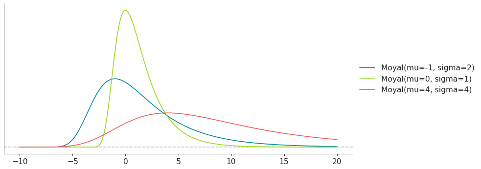

Support	$x \in (-\infty, \infty)$
Mean	$\mu + \sigma\left(\gamma + \log 2\right)$, where $\gamma$ is the Euler-Mascheroni constant
Variance	$\frac{\pi^{2}}{2}\sigma^{2}$

Parameters:

mu (float) – Location parameter.
sigma (float) – Scale parameter (sigma > 0).

cdf(x)[source]#

Cumulative distribution function.

Parameters:: x (array_like) – Values on which to evaluate the cdf

entropy()[source]#: Entropy.

eti(mass=None, fmt='.2f')#

Equal-tailed interval containing mass.

Parameters:

mass (float) – Probability mass in the interval. Defaults to None,
used. (which results in the value of rcParams["stats.ci_prob"] being)
fmt (str) – fmt used to represent results using f-string fmt for floats. Default to “.2f” i.e. 2 digits after the decimal point. Use “none” for no format.

hdi(mass=None, fmt='.2f')#

Highest density interval containing mass.

Parameters:

mass (float) – Probability mass in the interval. Defaults to None,
used. (which results in the value of rcParams["stats.ci_prob"] being)
fmt (str) – fmt used to represent results using f-string fmt for floats. Default to “.2f” i.e. 2 digits after the decimal point. Use “none” for no format.

isf(x)#

Inverse survival function (inverse of sf).

Parameters:: x (array_like) – Values on which to evaluate the inverse of the sf

kurtosis()[source]#: Excess kurtosis.

lmoment1()[source]#: L-moment1 (mean).

lmoment2()[source]#: L-moment2 (l-scale).

lmoment3()[source]#: L-moment3 (l-skewness). This the ratio of L-moment3 to L-moment2.

lmoment4()[source]#: L-moment4 (l-kurtosis). This the ratio of L-moment4 to L-moment2.

lmoments(types='1234')#

Compute L-moments of the distribution.

Parameters:: types (str) – The type of moments to compute. Default is ‘1234’ where ‘1’ = L-moment1 (mean), ‘2’ = L-moment2 (l-scale), ‘3’ = L-moment3 (l-skewness), and ‘4’ = L-moment4 (l-kurtosis). To compute the standard deviation use ‘d’ Valid combinations are any subset of ‘1234’.

logcdf(x)#

Log cumulative distribution function.

Parameters:: x (array_like) – Values on which to evaluate the logcdf

logpdf(x)[source]#

Log probability density/mass function.

Parameters:: x (array_like) – Values on which to evaluate the logpdf

logsf(x)#

Log survival function log(1 - cdf).

Parameters:: x (array_like) – Values on which to evaluate the logsf

mean()[source]#: Mean.

median()[source]#: Median.

mode()[source]#: Mode.

moments(types='mvsk')#

Compute moments of the distribution.

It can also return the standard deviation

Parameters:: types (str) – The type of moments to compute. Default is ‘mvsk’ where ‘m’ = mean, ‘v’ = variance, ‘s’ = skewness, and ‘k’ = kurtosis. To compute the standard deviation use ‘d’ Valid combinations are any subset of ‘mvdsk’.

pdf(x)[source]#

Probability density/mass function.

Parameters:: x (array_like) – Values on which to evaluate the pdf

plot_cdf(moments=None, pointinterval=False, interval=None, levels=None, support='restricted', legend='legend', figsize=None, ax=None, **kwargs)#

Plot the cumulative distribution function.

Parameters:

moments (str) – Compute moments. Use any combination of the strings m, d, v, s or k for the mean (μ), standard deviation (σ), variance (σ²), skew (γ) or kurtosis (κ) respectively. Other strings will be ignored. Defaults to None.
pointinterval (bool) – Whether to include a plot of the quantiles. Defaults to False. If True the default is to plot the median and two interquantiles ranges.
interval (str) – Type of interval. Available options are highest density interval “hdi” (default), equal tailed interval “eti” or intervals defined by arbitrary “quantiles”. Defaults to the value in rcParams[“stats.ci_kind”].
levels (list) – Mass of the intervals. For hdi or eti the number of elements should be 2 or 1. For quantiles the number of elements should be 5, 3, 1 or 0 (in this last case nothing will be plotted).
support (str:) – If full use the finite end-points to set the limits of the plot. For unbounded end-points or if restricted use the 0.001 and 0.999 quantiles to set the limits.
legend (str) – Whether to include a string with the distribution and its parameter as a "legend" a "title" or not include them None.
figsize (tuple) – Size of the figure
ax (matplotlib axes)
kwargs (keyword arguments) – Additional keyword arguments passed to matplotlib plot function. For example, color, alpha, linewidth, etc.

plot_interactive(kind='pdf', xy_lim='both', pointinterval=True, interval=None, levels=None, figsize=None)#

Interactive exploration of distributions parameters.

Parameters:

kind (str:) – Type of plot. Available options are pdf, cdf and ppf.
xy_lim (str or tuple) – Set the limits of the x-axis and/or y-axis. Defaults to “both”, the limits of both axis are fixed. Use “auto” for automatic rescaling of x-axis and y-axis. Or set them manually by passing a tuple of 4 elements, the first two for x-axis, the last two for y-axis. The tuple can have None.
pointinterval (bool) – Whether to include a plot of the quantiles. Defaults to False. If True the default is to plot the median and two interquantiles ranges.
interval (str) – Type of interval. Available options are highest density interval “hdi” (default), equal tailed interval “eti” or intervals defined by arbitrary “quantiles”. Defaults to the value in rcParams[“stats.ci_kind”].
levels (list) – Mass of the intervals. For hdi or eti the number of elements should be 2 or 1. For quantiles the number of elements should be 5, 3, 1 or 0 (in this last case nothing will be plotted).
figsize (tuple) – Size of the figure

plot_isf(moments=None, pointinterval=False, interval=None, levels=None, legend='legend', figsize=None, ax=None, **kwargs)#

Plot the inverse survival function.

Parameters:

moments (str) – Compute moments. Use any combination of the strings m, d, v, s or k for the mean (μ), standard deviation (σ), variance (σ²), skew (γ) or kurtosis (κ) respectively. Other strings will be ignored. Defaults to None.
pointinterval (bool) – Whether to include a plot of the quantiles. Defaults to False. If True the default is to plot the median and two interquantiles ranges.
interval (str) – Type of interval. Available options are highest density interval “hdi” (default), equal tailed interval “eti” or intervals defined by arbitrary “quantiles”. Defaults to the value in rcParams[“stats.ci_kind”].
levels (list) – Mass of the intervals. For hdi or eti the number of elements should be 2 or 1. For quantiles the number of elements should be 5, 3, 1 or 0 (in this last case nothing will be plotted).
legend (str) – Whether to include a string with the distribution and its parameter as a "legend" a "title" or not include them None.
figsize (tuple) – Size of the figure
ax (matplotlib axes)

plot_pdf(moments=None, pointinterval=False, interval=None, levels=None, support='restricted', baseline=True, legend='legend', figsize=None, ax=None, **kwargs)#

Plot the pdf (continuous) or pmf (discrete).

Parameters:

moments (str) – Compute moments. Use any combination of the strings m, d, v, s or k for the mean (μ), standard deviation (σ), variance (σ²), skew (γ) or kurtosis (κ) respectively. Other strings will be ignored. Defaults to None.
pointinterval (bool) – Whether to include a plot of the quantiles. Defaults to False. If True the default is to plot the median and two interquantiles ranges.
interval (str) – Type of interval. Available options are highest density interval “hdi” (default), equal tailed interval “eti” or intervals defined by arbitrary “quantiles”. Defaults to the value in rcParams[“stats.ci_kind”].
levels (list) – Mass of the intervals. For hdi or eti the number of elements should be 2 or 1. For quantiles the number of elements should be 5, 3, 1 or 0 (in this last case nothing will be plotted).
support (str:) – If full use the finite end-points to set the limits of the plot. For unbounded end-points or if restricted use the 0.001 and 0.999 quantiles to set the limits.
baseline (bool) – Whether to include a horizontal line at y=0.
legend (str) – Whether to include a string with the distribution and its parameter as a "legend" a "title" or not include them None.
figsize (tuple) – Size of the figure
ax (matplotlib axes)
kwargs (keyword arguments) – Additional keyword arguments passed to matplotlib plot function. For example, color, alpha, linewidth, etc.

plot_ppf(moments=None, pointinterval=False, interval=None, levels=None, legend='legend', figsize=None, ax=None, **kwargs)#

Plot the quantile function.

Parameters:

moments (str) – Compute moments. Use any combination of the strings m, d, v, s or k for the mean (μ), standard deviation (σ), variance (σ²), skew (γ) or kurtosis (κ) respectively. Other strings will be ignored. Defaults to None.
pointinterval (bool) – Whether to include a plot of the quantiles. Defaults to False. If True the default is to plot the median and two interquantiles ranges.
interval (str) – Type of interval. Available options are highest density interval “hdi” (default), equal tailed interval “eti” or intervals defined by arbitrary “quantiles”. Defaults to the value in rcParams[“stats.ci_kind”].
levels (list) – Mass of the intervals. For hdi or eti the number of elements should be 2 or 1. For quantiles the number of elements should be 5, 3, 1 or 0 (in this last case nothing will be plotted).
legend (str) – Whether to include a string with the distribution and its parameter as a "legend" a "title" or not include them None.
figsize (tuple) – Size of the figure
ax (matplotlib axes)

plot_sf(moments=None, pointinterval=False, interval=None, levels=None, support='restricted', legend='legend', figsize=None, ax=None, **kwargs)#

Plot the survival distribution function (1 - CDF).

Parameters:

moments (str) – Compute moments. Use any combination of the strings m, d, v, s or k for the mean (μ), standard deviation (σ), variance (σ²), skew (γ) or kurtosis (κ) respectively. Other strings will be ignored. Defaults to None.
pointinterval (bool) – Whether to include a plot of the quantiles. Defaults to False. If True the default is to plot the median and two interquantiles ranges.
interval (str) – Type of interval. Available options are highest density interval “hdi” (default), equal tailed interval “eti” or intervals defined by arbitrary “quantiles”. Defaults to the value in rcParams[“stats.ci_kind”].
levels (list) – Mass of the intervals. For hdi or eti the number of elements should be 2 or 1. For quantiles the number of elements should be 5, 3, 1 or 0 (in this last case nothing will be plotted).
support (str:) – If full use the finite end-points to set the limits of the plot. For unbounded end-points or if restricted use the 0.001 and 0.999 quantiles to set the limits.
legend (str) – Whether to include a string with the distribution and its parameter as a "legend" a "title" or not include them None.
figsize (tuple) – Size of the figure
ax (matplotlib axes)
kwargs (keyword arguments) – Additional keyword arguments passed to matplotlib plot function. For example, color, alpha, linewidth, etc.

ppf(q)[source]#

Percent point function (inverse of cdf).

Parameters:: x (array_like) – Values on which to evaluate the inverse of the cdf

rvs(size=None, random_state=None)[source]#

Random sample.

Parameters:

size (int or tuple of ints, optional) – Defining number of random variates. Defaults to 1.
random_state ({None, int, numpy.random.Generator, numpy.random.RandomState}) – Defaults to None

sf(x)#

Survival function (1 - cdf).

Parameters:: x (array_like) – Values on which to evaluate the sf

skewness()[source]#: Skewness.

std()[source]#: Standard deviation.

summary(mass=None, interval=None, fmt='.2f')#

Namedtuple with the mean, median, sd, and lower and upper bounds.

Parameters:

mass (float) – Probability mass for the equal-tailed interval. Defaults to None,
used. (which results in the value of rcParams["stats.ci_prob"] being)
interval (str or list-like) – Type of interval. Available options are highest density interval “hdi”, equal tailed interval “eti” or arbitrary interval defined by a list-like object with a pair of values. Defaults to the value in rcParams[“stats.ci_kind”].
fmt (str) – fmt used to represent results using f-string fmt for floats. Default to “.2f” i.e. 2 digits after the decimal point.

to_bambi(**kwargs)#

Convert the PreliZ distribution to a Bambi Prior.

kwargsPyMC distributions properties: kwargs are used to specify properties such as shape or dims

Return type:: Bambi Prior

to_pymc(name=None, **kwargs)#

Convert the PreliZ distribution to a PyMC distribution.

namestr: Name of PyMC distribution. Needed if inside Model context
kwargsPyMC distributions properties: kwargs are used to specify properties such as shape or dims

Return type:: PyMC distribution

var()[source]#: Variance.

xvals(support, n_points=None)#

Provide x values in the support of the distribution.

This is useful for example when plotting.

Parameters:

support (str) – Available options are “full” or “restricted”. If “full” the values will cover the entire support of the distribution if the boundary is finite, or the quantiles 0.0001 or 0.9999, if infinite. If “restricted” the values will cover the quantile 0.0001 to 0.9999.
n_points (int) – Number of values to return. Defaults to 1000 for continuous distributions and 200 for discrete ones. For discrete distributions the returned values may be fewer than n_points if the actual number of discrete values in the support of the distribution is smaller than n_points.

class preliz.distributions.normal.Normal(mu=None, sigma=None, tau=None)[source]#

Normal distribution.

The pdf of this distribution is

\[f(x \mid \mu, \sigma) = \frac{1}{\sigma \sqrt{2\pi}} \exp\left\{ -\frac{1}{2} \left(\frac{x-\mu}{\sigma}\right)^2 \right\}\]

(Source code, png, hires.png, pdf)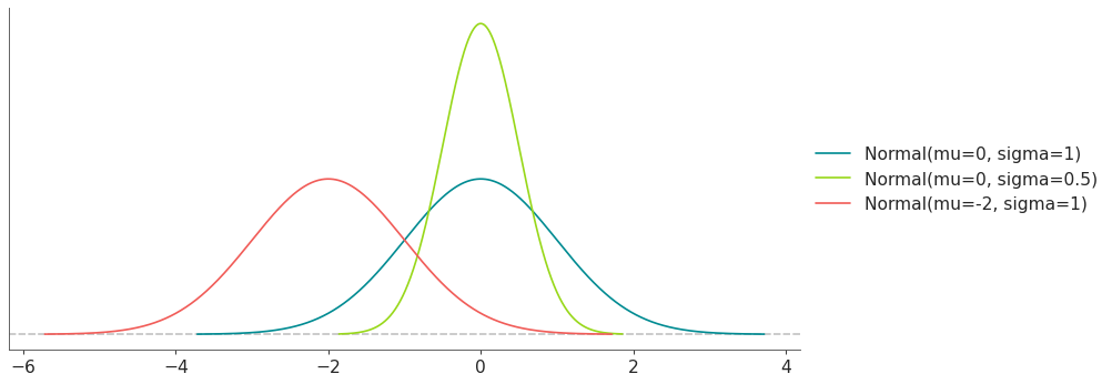

Support	$x \in \mathbb{R}$
Mean	$\mu$
Variance	$\sigma^2$

Normal distribution has 2 alternative parameterizations. In terms of mean and sigma (standard deviation), or mean and tau (precision).

The link between the 2 alternatives is given by

\[\tau = \frac{1}{\sigma^2}\]

Parameters:

mu (float) – Mean.
sigma (float) – Standard deviation (sigma > 0).
tau (float) – Precision (tau > 0).

cdf(x)[source]#

Cumulative distribution function.

Parameters:: x (array_like) – Values on which to evaluate the cdf

entropy()[source]#: Entropy.

eti(mass=None, fmt='.2f')#

Equal-tailed interval containing mass.

Parameters:

mass (float) – Probability mass in the interval. Defaults to None,
used. (which results in the value of rcParams["stats.ci_prob"] being)
fmt (str) – fmt used to represent results using f-string fmt for floats. Default to “.2f” i.e. 2 digits after the decimal point. Use “none” for no format.

hdi(mass=None, fmt='.2f')#

Highest density interval containing mass.

Parameters:

mass (float) – Probability mass in the interval. Defaults to None,
used. (which results in the value of rcParams["stats.ci_prob"] being)
fmt (str) – fmt used to represent results using f-string fmt for floats. Default to “.2f” i.e. 2 digits after the decimal point. Use “none” for no format.

isf(q)[source]#

Inverse survival function (inverse of sf).

Parameters:: x (array_like) – Values on which to evaluate the inverse of the sf

kurtosis()[source]#: Excess kurtosis.

lmoment1()[source]#: L-moment1 (mean).

lmoment2()[source]#: L-moment2 (l-scale).

lmoment3()[source]#: L-moment3 (l-skewness). This the ratio of L-moment3 to L-moment2.

lmoment4()[source]#: L-moment4 (l-kurtosis). This the ratio of L-moment4 to L-moment2.

lmoments(types='1234')#

Compute L-moments of the distribution.

Parameters:: types (str) – The type of moments to compute. Default is ‘1234’ where ‘1’ = L-moment1 (mean), ‘2’ = L-moment2 (l-scale), ‘3’ = L-moment3 (l-skewness), and ‘4’ = L-moment4 (l-kurtosis). To compute the standard deviation use ‘d’ Valid combinations are any subset of ‘1234’.

logcdf(x)[source]#

Log cumulative distribution function.

Parameters:: x (array_like) – Values on which to evaluate the logcdf

logpdf(x)[source]#

Log probability density/mass function.

Parameters:: x (array_like) – Values on which to evaluate the logpdf

logsf(x)[source]#

Log survival function log(1 - cdf).

Parameters:: x (array_like) – Values on which to evaluate the logsf

mean()[source]#: Mean.

median()[source]#: Median.

mode()[source]#: Mode.

moments(types='mvsk')#

Compute moments of the distribution.

It can also return the standard deviation

Parameters:: types (str) – The type of moments to compute. Default is ‘mvsk’ where ‘m’ = mean, ‘v’ = variance, ‘s’ = skewness, and ‘k’ = kurtosis. To compute the standard deviation use ‘d’ Valid combinations are any subset of ‘mvdsk’.

pdf(x)[source]#

Probability density/mass function.

Parameters:: x (array_like) – Values on which to evaluate the pdf

plot_cdf(moments=None, pointinterval=False, interval=None, levels=None, support='restricted', legend='legend', figsize=None, ax=None, **kwargs)#

Plot the cumulative distribution function.

Parameters:

moments (str) – Compute moments. Use any combination of the strings m, d, v, s or k for the mean (μ), standard deviation (σ), variance (σ²), skew (γ) or kurtosis (κ) respectively. Other strings will be ignored. Defaults to None.
pointinterval (bool) – Whether to include a plot of the quantiles. Defaults to False. If True the default is to plot the median and two interquantiles ranges.
interval (str) – Type of interval. Available options are highest density interval “hdi” (default), equal tailed interval “eti” or intervals defined by arbitrary “quantiles”. Defaults to the value in rcParams[“stats.ci_kind”].
levels (list) – Mass of the intervals. For hdi or eti the number of elements should be 2 or 1. For quantiles the number of elements should be 5, 3, 1 or 0 (in this last case nothing will be plotted).
support (str:) – If full use the finite end-points to set the limits of the plot. For unbounded end-points or if restricted use the 0.001 and 0.999 quantiles to set the limits.
legend (str) – Whether to include a string with the distribution and its parameter as a "legend" a "title" or not include them None.
figsize (tuple) – Size of the figure
ax (matplotlib axes)
kwargs (keyword arguments) – Additional keyword arguments passed to matplotlib plot function. For example, color, alpha, linewidth, etc.

plot_interactive(kind='pdf', xy_lim='both', pointinterval=True, interval=None, levels=None, figsize=None)#

Interactive exploration of distributions parameters.

Parameters:

kind (str:) – Type of plot. Available options are pdf, cdf and ppf.
xy_lim (str or tuple) – Set the limits of the x-axis and/or y-axis. Defaults to “both”, the limits of both axis are fixed. Use “auto” for automatic rescaling of x-axis and y-axis. Or set them manually by passing a tuple of 4 elements, the first two for x-axis, the last two for y-axis. The tuple can have None.
pointinterval (bool) – Whether to include a plot of the quantiles. Defaults to False. If True the default is to plot the median and two interquantiles ranges.
interval (str) – Type of interval. Available options are highest density interval “hdi” (default), equal tailed interval “eti” or intervals defined by arbitrary “quantiles”. Defaults to the value in rcParams[“stats.ci_kind”].
levels (list) – Mass of the intervals. For hdi or eti the number of elements should be 2 or 1. For quantiles the number of elements should be 5, 3, 1 or 0 (in this last case nothing will be plotted).
figsize (tuple) – Size of the figure

plot_isf(moments=None, pointinterval=False, interval=None, levels=None, legend='legend', figsize=None, ax=None, **kwargs)#

Plot the inverse survival function.

Parameters:

moments (str) – Compute moments. Use any combination of the strings m, d, v, s or k for the mean (μ), standard deviation (σ), variance (σ²), skew (γ) or kurtosis (κ) respectively. Other strings will be ignored. Defaults to None.
pointinterval (bool) – Whether to include a plot of the quantiles. Defaults to False. If True the default is to plot the median and two interquantiles ranges.
interval (str) – Type of interval. Available options are highest density interval “hdi” (default), equal tailed interval “eti” or intervals defined by arbitrary “quantiles”. Defaults to the value in rcParams[“stats.ci_kind”].
levels (list) – Mass of the intervals. For hdi or eti the number of elements should be 2 or 1. For quantiles the number of elements should be 5, 3, 1 or 0 (in this last case nothing will be plotted).
legend (str) – Whether to include a string with the distribution and its parameter as a "legend" a "title" or not include them None.
figsize (tuple) – Size of the figure
ax (matplotlib axes)

plot_pdf(moments=None, pointinterval=False, interval=None, levels=None, support='restricted', baseline=True, legend='legend', figsize=None, ax=None, **kwargs)#

Plot the pdf (continuous) or pmf (discrete).

Parameters:

moments (str) – Compute moments. Use any combination of the strings m, d, v, s or k for the mean (μ), standard deviation (σ), variance (σ²), skew (γ) or kurtosis (κ) respectively. Other strings will be ignored. Defaults to None.
pointinterval (bool) – Whether to include a plot of the quantiles. Defaults to False. If True the default is to plot the median and two interquantiles ranges.
interval (str) – Type of interval. Available options are highest density interval “hdi” (default), equal tailed interval “eti” or intervals defined by arbitrary “quantiles”. Defaults to the value in rcParams[“stats.ci_kind”].
levels (list) – Mass of the intervals. For hdi or eti the number of elements should be 2 or 1. For quantiles the number of elements should be 5, 3, 1 or 0 (in this last case nothing will be plotted).
support (str:) – If full use the finite end-points to set the limits of the plot. For unbounded end-points or if restricted use the 0.001 and 0.999 quantiles to set the limits.
baseline (bool) – Whether to include a horizontal line at y=0.
legend (str) – Whether to include a string with the distribution and its parameter as a "legend" a "title" or not include them None.
figsize (tuple) – Size of the figure
ax (matplotlib axes)
kwargs (keyword arguments) – Additional keyword arguments passed to matplotlib plot function. For example, color, alpha, linewidth, etc.

plot_ppf(moments=None, pointinterval=False, interval=None, levels=None, legend='legend', figsize=None, ax=None, **kwargs)#

Plot the quantile function.

Parameters:

moments (str) – Compute moments. Use any combination of the strings m, d, v, s or k for the mean (μ), standard deviation (σ), variance (σ²), skew (γ) or kurtosis (κ) respectively. Other strings will be ignored. Defaults to None.
pointinterval (bool) – Whether to include a plot of the quantiles. Defaults to False. If True the default is to plot the median and two interquantiles ranges.
interval (str) – Type of interval. Available options are highest density interval “hdi” (default), equal tailed interval “eti” or intervals defined by arbitrary “quantiles”. Defaults to the value in rcParams[“stats.ci_kind”].
levels (list) – Mass of the intervals. For hdi or eti the number of elements should be 2 or 1. For quantiles the number of elements should be 5, 3, 1 or 0 (in this last case nothing will be plotted).
legend (str) – Whether to include a string with the distribution and its parameter as a "legend" a "title" or not include them None.
figsize (tuple) – Size of the figure
ax (matplotlib axes)

plot_sf(moments=None, pointinterval=False, interval=None, levels=None, support='restricted', legend='legend', figsize=None, ax=None, **kwargs)#

Plot the survival distribution function (1 - CDF).

Parameters:

moments (str) – Compute moments. Use any combination of the strings m, d, v, s or k for the mean (μ), standard deviation (σ), variance (σ²), skew (γ) or kurtosis (κ) respectively. Other strings will be ignored. Defaults to None.
pointinterval (bool) – Whether to include a plot of the quantiles. Defaults to False. If True the default is to plot the median and two interquantiles ranges.
interval (str) – Type of interval. Available options are highest density interval “hdi” (default), equal tailed interval “eti” or intervals defined by arbitrary “quantiles”. Defaults to the value in rcParams[“stats.ci_kind”].
levels (list) – Mass of the intervals. For hdi or eti the number of elements should be 2 or 1. For quantiles the number of elements should be 5, 3, 1 or 0 (in this last case nothing will be plotted).
support (str:) – If full use the finite end-points to set the limits of the plot. For unbounded end-points or if restricted use the 0.001 and 0.999 quantiles to set the limits.
legend (str) – Whether to include a string with the distribution and its parameter as a "legend" a "title" or not include them None.
figsize (tuple) – Size of the figure
ax (matplotlib axes)
kwargs (keyword arguments) – Additional keyword arguments passed to matplotlib plot function. For example, color, alpha, linewidth, etc.

ppf(q)[source]#

Percent point function (inverse of cdf).

Parameters:: x (array_like) – Values on which to evaluate the inverse of the cdf

rvs(size=None, random_state=None)[source]#

Random sample.

Parameters:

size (int or tuple of ints, optional) – Defining number of random variates. Defaults to 1.
random_state ({None, int, numpy.random.Generator, numpy.random.RandomState}) – Defaults to None

sf(x)[source]#

Survival function (1 - cdf).

Parameters:: x (array_like) – Values on which to evaluate the sf

skewness()[source]#: Skewness.

std()[source]#: Standard deviation.

summary(mass=None, interval=None, fmt='.2f')#

Namedtuple with the mean, median, sd, and lower and upper bounds.

Parameters:

mass (float) – Probability mass for the equal-tailed interval. Defaults to None,
used. (which results in the value of rcParams["stats.ci_prob"] being)
interval (str or list-like) – Type of interval. Available options are highest density interval “hdi”, equal tailed interval “eti” or arbitrary interval defined by a list-like object with a pair of values. Defaults to the value in rcParams[“stats.ci_kind”].
fmt (str) – fmt used to represent results using f-string fmt for floats. Default to “.2f” i.e. 2 digits after the decimal point.

to_bambi(**kwargs)#

Convert the PreliZ distribution to a Bambi Prior.

kwargsPyMC distributions properties: kwargs are used to specify properties such as shape or dims

Return type:: Bambi Prior

to_pymc(name=None, **kwargs)#

Convert the PreliZ distribution to a PyMC distribution.

namestr: Name of PyMC distribution. Needed if inside Model context
kwargsPyMC distributions properties: kwargs are used to specify properties such as shape or dims

Return type:: PyMC distribution

var()[source]#: Variance.

xvals(support, n_points=None)#

Provide x values in the support of the distribution.

This is useful for example when plotting.

Parameters:

support (str) – Available options are “full” or “restricted”. If “full” the values will cover the entire support of the distribution if the boundary is finite, or the quantiles 0.0001 or 0.9999, if infinite. If “restricted” the values will cover the quantile 0.0001 to 0.9999.
n_points (int) – Number of values to return. Defaults to 1000 for continuous distributions and 200 for discrete ones. For discrete distributions the returned values may be fewer than n_points if the actual number of discrete values in the support of the distribution is smaller than n_points.

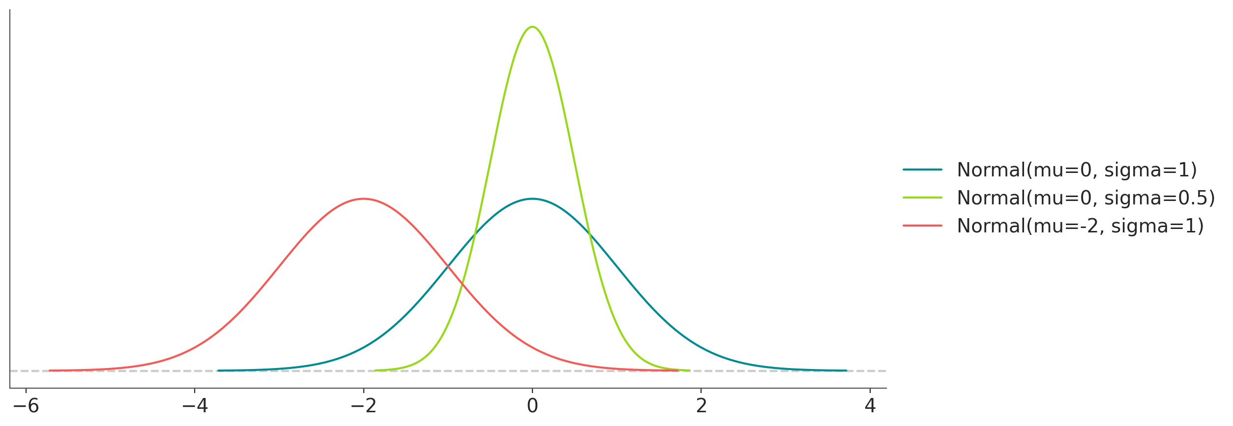
class preliz.distributions.pareto.Pareto(alpha=None, m=None)[source]#

Pareto distribution.

The pdf of this distribution is

\[f(x \mid \alpha, m) = \frac{\alpha m^{\alpha}}{x^{\alpha+1}}\]

(Source code, png, hires.png, pdf)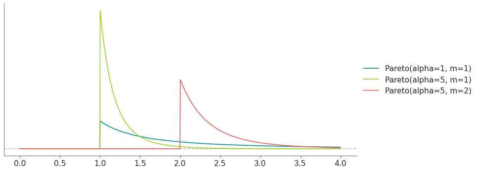

Support	$x \in [m, \infty)$
Mean	$\dfrac{\alpha m}{\alpha - 1}$ for $\alpha \ge 1$
Variance	$\dfrac{m^2 \alpha}{(\alpha - 1)^2 (\alpha - 2)}$ for $\alpha > 2$

Parameters:

alpha (float) – Shape parameter (alpha > 0).
m (float) – Scale parameter (m > 0).

cdf(x)[source]#

Cumulative distribution function.

Parameters:: x (array_like) – Values on which to evaluate the cdf

entropy()[source]#: Entropy.

eti(mass=None, fmt='.2f')#

Equal-tailed interval containing mass.

Parameters:

mass (float) – Probability mass in the interval. Defaults to None,
used. (which results in the value of rcParams["stats.ci_prob"] being)
fmt (str) – fmt used to represent results using f-string fmt for floats. Default to “.2f” i.e. 2 digits after the decimal point. Use “none” for no format.

hdi(mass=None, fmt='.2f')#

Highest density interval containing mass.

Parameters:

mass (float) – Probability mass in the interval. Defaults to None,
used. (which results in the value of rcParams["stats.ci_prob"] being)
fmt (str) – fmt used to represent results using f-string fmt for floats. Default to “.2f” i.e. 2 digits after the decimal point. Use “none” for no format.

isf(x)#

Inverse survival function (inverse of sf).

Parameters:: x (array_like) – Values on which to evaluate the inverse of the sf

kurtosis()[source]#: Excess kurtosis.

lmoment1()[source]#: L-moment1 (mean).

lmoment2()[source]#: L-moment2 (l-scale).

lmoment3()[source]#: L-moment3 (l-skewness). This the ratio of L-moment3 to L-moment2.

lmoment4()[source]#: L-moment4 (l-kurtosis). This the ratio of L-moment4 to L-moment2.

lmoments(types='1234')#

Compute L-moments of the distribution.

Parameters:: types (str) – The type of moments to compute. Default is ‘1234’ where ‘1’ = L-moment1 (mean), ‘2’ = L-moment2 (l-scale), ‘3’ = L-moment3 (l-skewness), and ‘4’ = L-moment4 (l-kurtosis). To compute the standard deviation use ‘d’ Valid combinations are any subset of ‘1234’.

logcdf(x)#

Log cumulative distribution function.

Parameters:: x (array_like) – Values on which to evaluate the logcdf

logpdf(x)[source]#

Log probability density/mass function.

Parameters:: x (array_like) – Values on which to evaluate the logpdf

logsf(x)#

Log survival function log(1 - cdf).

Parameters:: x (array_like) – Values on which to evaluate the logsf

mean()[source]#: Mean.

median()[source]#: Median.

mode()[source]#: Mode.

moments(types='mvsk')#

Compute moments of the distribution.

It can also return the standard deviation

Parameters:: types (str) – The type of moments to compute. Default is ‘mvsk’ where ‘m’ = mean, ‘v’ = variance, ‘s’ = skewness, and ‘k’ = kurtosis. To compute the standard deviation use ‘d’ Valid combinations are any subset of ‘mvdsk’.

pdf(x)[source]#

Probability density/mass function.

Parameters:: x (array_like) – Values on which to evaluate the pdf

plot_cdf(moments=None, pointinterval=False, interval=None, levels=None, support='restricted', legend='legend', figsize=None, ax=None, **kwargs)#

Plot the cumulative distribution function.

Parameters:

moments (str) – Compute moments. Use any combination of the strings m, d, v, s or k for the mean (μ), standard deviation (σ), variance (σ²), skew (γ) or kurtosis (κ) respectively. Other strings will be ignored. Defaults to None.
pointinterval (bool) – Whether to include a plot of the quantiles. Defaults to False. If True the default is to plot the median and two interquantiles ranges.
interval (str) – Type of interval. Available options are highest density interval “hdi” (default), equal tailed interval “eti” or intervals defined by arbitrary “quantiles”. Defaults to the value in rcParams[“stats.ci_kind”].
levels (list) – Mass of the intervals. For hdi or eti the number of elements should be 2 or 1. For quantiles the number of elements should be 5, 3, 1 or 0 (in this last case nothing will be plotted).
support (str:) – If full use the finite end-points to set the limits of the plot. For unbounded end-points or if restricted use the 0.001 and 0.999 quantiles to set the limits.
legend (str) – Whether to include a string with the distribution and its parameter as a "legend" a "title" or not include them None.
figsize (tuple) – Size of the figure
ax (matplotlib axes)
kwargs (keyword arguments) – Additional keyword arguments passed to matplotlib plot function. For example, color, alpha, linewidth, etc.

plot_interactive(kind='pdf', xy_lim='both', pointinterval=True, interval=None, levels=None, figsize=None)#

Interactive exploration of distributions parameters.

Parameters:

kind (str:) – Type of plot. Available options are pdf, cdf and ppf.
xy_lim (str or tuple) – Set the limits of the x-axis and/or y-axis. Defaults to “both”, the limits of both axis are fixed. Use “auto” for automatic rescaling of x-axis and y-axis. Or set them manually by passing a tuple of 4 elements, the first two for x-axis, the last two for y-axis. The tuple can have None.
pointinterval (bool) – Whether to include a plot of the quantiles. Defaults to False. If True the default is to plot the median and two interquantiles ranges.
interval (str) – Type of interval. Available options are highest density interval “hdi” (default), equal tailed interval “eti” or intervals defined by arbitrary “quantiles”. Defaults to the value in rcParams[“stats.ci_kind”].
levels (list) – Mass of the intervals. For hdi or eti the number of elements should be 2 or 1. For quantiles the number of elements should be 5, 3, 1 or 0 (in this last case nothing will be plotted).
figsize (tuple) – Size of the figure

plot_isf(moments=None, pointinterval=False, interval=None, levels=None, legend='legend', figsize=None, ax=None, **kwargs)#

Plot the inverse survival function.

Parameters:

moments (str) – Compute moments. Use any combination of the strings m, d, v, s or k for the mean (μ), standard deviation (σ), variance (σ²), skew (γ) or kurtosis (κ) respectively. Other strings will be ignored. Defaults to None.
pointinterval (bool) – Whether to include a plot of the quantiles. Defaults to False. If True the default is to plot the median and two interquantiles ranges.
interval (str) – Type of interval. Available options are highest density interval “hdi” (default), equal tailed interval “eti” or intervals defined by arbitrary “quantiles”. Defaults to the value in rcParams[“stats.ci_kind”].
levels (list) – Mass of the intervals. For hdi or eti the number of elements should be 2 or 1. For quantiles the number of elements should be 5, 3, 1 or 0 (in this last case nothing will be plotted).
legend (str) – Whether to include a string with the distribution and its parameter as a "legend" a "title" or not include them None.
figsize (tuple) – Size of the figure
ax (matplotlib axes)

plot_pdf(moments=None, pointinterval=False, interval=None, levels=None, support='restricted', baseline=True, legend='legend', figsize=None, ax=None, **kwargs)#

Plot the pdf (continuous) or pmf (discrete).

Parameters:

moments (str) – Compute moments. Use any combination of the strings m, d, v, s or k for the mean (μ), standard deviation (σ), variance (σ²), skew (γ) or kurtosis (κ) respectively. Other strings will be ignored. Defaults to None.
pointinterval (bool) – Whether to include a plot of the quantiles. Defaults to False. If True the default is to plot the median and two interquantiles ranges.
interval (str) – Type of interval. Available options are highest density interval “hdi” (default), equal tailed interval “eti” or intervals defined by arbitrary “quantiles”. Defaults to the value in rcParams[“stats.ci_kind”].
levels (list) – Mass of the intervals. For hdi or eti the number of elements should be 2 or 1. For quantiles the number of elements should be 5, 3, 1 or 0 (in this last case nothing will be plotted).
support (str:) – If full use the finite end-points to set the limits of the plot. For unbounded end-points or if restricted use the 0.001 and 0.999 quantiles to set the limits.
baseline (bool) – Whether to include a horizontal line at y=0.
legend (str) – Whether to include a string with the distribution and its parameter as a "legend" a "title" or not include them None.
figsize (tuple) – Size of the figure
ax (matplotlib axes)
kwargs (keyword arguments) – Additional keyword arguments passed to matplotlib plot function. For example, color, alpha, linewidth, etc.

plot_ppf(moments=None, pointinterval=False, interval=None, levels=None, legend='legend', figsize=None, ax=None, **kwargs)#

Plot the quantile function.

Parameters:

moments (str) – Compute moments. Use any combination of the strings m, d, v, s or k for the mean (μ), standard deviation (σ), variance (σ²), skew (γ) or kurtosis (κ) respectively. Other strings will be ignored. Defaults to None.
pointinterval (bool) – Whether to include a plot of the quantiles. Defaults to False. If True the default is to plot the median and two interquantiles ranges.
interval (str) – Type of interval. Available options are highest density interval “hdi” (default), equal tailed interval “eti” or intervals defined by arbitrary “quantiles”. Defaults to the value in rcParams[“stats.ci_kind”].
levels (list) – Mass of the intervals. For hdi or eti the number of elements should be 2 or 1. For quantiles the number of elements should be 5, 3, 1 or 0 (in this last case nothing will be plotted).
legend (str) – Whether to include a string with the distribution and its parameter as a "legend" a "title" or not include them None.
figsize (tuple) – Size of the figure
ax (matplotlib axes)

plot_sf(moments=None, pointinterval=False, interval=None, levels=None, support='restricted', legend='legend', figsize=None, ax=None, **kwargs)#

Plot the survival distribution function (1 - CDF).

Parameters:

moments (str) – Compute moments. Use any combination of the strings m, d, v, s or k for the mean (μ), standard deviation (σ), variance (σ²), skew (γ) or kurtosis (κ) respectively. Other strings will be ignored. Defaults to None.
pointinterval (bool) – Whether to include a plot of the quantiles. Defaults to False. If True the default is to plot the median and two interquantiles ranges.
interval (str) – Type of interval. Available options are highest density interval “hdi” (default), equal tailed interval “eti” or intervals defined by arbitrary “quantiles”. Defaults to the value in rcParams[“stats.ci_kind”].
levels (list) – Mass of the intervals. For hdi or eti the number of elements should be 2 or 1. For quantiles the number of elements should be 5, 3, 1 or 0 (in this last case nothing will be plotted).
support (str:) – If full use the finite end-points to set the limits of the plot. For unbounded end-points or if restricted use the 0.001 and 0.999 quantiles to set the limits.
legend (str) – Whether to include a string with the distribution and its parameter as a "legend" a "title" or not include them None.
figsize (tuple) – Size of the figure
ax (matplotlib axes)
kwargs (keyword arguments) – Additional keyword arguments passed to matplotlib plot function. For example, color, alpha, linewidth, etc.

ppf(q)[source]#

Percent point function (inverse of cdf).

Parameters:: x (array_like) – Values on which to evaluate the inverse of the cdf

rvs(size=None, random_state=None)[source]#

Random sample.

Parameters:

size (int or tuple of ints, optional) – Defining number of random variates. Defaults to 1.
random_state ({None, int, numpy.random.Generator, numpy.random.RandomState}) – Defaults to None

sf(x)#

Survival function (1 - cdf).

Parameters:: x (array_like) – Values on which to evaluate the sf

skewness()[source]#: Skewness.

std()[source]#: Standard deviation.

summary(mass=None, interval=None, fmt='.2f')#

Namedtuple with the mean, median, sd, and lower and upper bounds.

Parameters:

mass (float) – Probability mass for the equal-tailed interval. Defaults to None,
used. (which results in the value of rcParams["stats.ci_prob"] being)
interval (str or list-like) – Type of interval. Available options are highest density interval “hdi”, equal tailed interval “eti” or arbitrary interval defined by a list-like object with a pair of values. Defaults to the value in rcParams[“stats.ci_kind”].
fmt (str) – fmt used to represent results using f-string fmt for floats. Default to “.2f” i.e. 2 digits after the decimal point.

to_bambi(**kwargs)#

Convert the PreliZ distribution to a Bambi Prior.

kwargsPyMC distributions properties: kwargs are used to specify properties such as shape or dims

Return type:: Bambi Prior

to_pymc(name=None, **kwargs)#

Convert the PreliZ distribution to a PyMC distribution.

namestr: Name of PyMC distribution. Needed if inside Model context
kwargsPyMC distributions properties: kwargs are used to specify properties such as shape or dims

Return type:: PyMC distribution

var()[source]#: Variance.

xvals(support, n_points=None)#

Provide x values in the support of the distribution.

This is useful for example when plotting.

Parameters:

support (str) – Available options are “full” or “restricted”. If “full” the values will cover the entire support of the distribution if the boundary is finite, or the quantiles 0.0001 or 0.9999, if infinite. If “restricted” the values will cover the quantile 0.0001 to 0.9999.
n_points (int) – Number of values to return. Defaults to 1000 for continuous distributions and 200 for discrete ones. For discrete distributions the returned values may be fewer than n_points if the actual number of discrete values in the support of the distribution is smaller than n_points.

class preliz.distributions.rice.Rice(nu=None, sigma=None, b=None)[source]#

Rice distribution.

The pdf of this distribution is

\[f(x\mid \nu ,\sigma )= {\frac {x}{\sigma ^{2}}}\exp \left({\frac {-(x^{2}+\nu ^{2})} {2\sigma ^{2}}}\right)I_{0}\left({\frac {x\nu }{\sigma ^{2}}}\right)\]

(Source code, png, hires.png, pdf)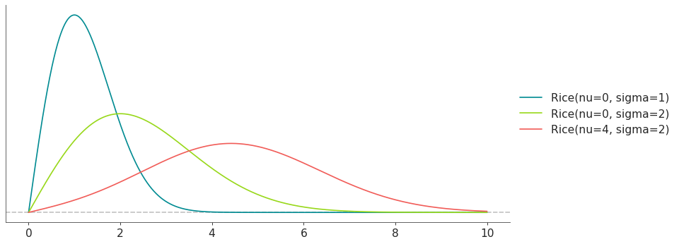

Support	$x \in (0, \infty)$
Mean	$\sigma \sqrt{\pi /2} L_{1/2}(-\nu^2 / 2\sigma^2)$
Variance	$2\sigma^2 + \nu^2 - \frac{\pi \sigma^2}{2}$ $L_{1/2}^2\left(\frac{-\nu^2}{2\sigma^2}\right)$

Rice distribution has 2 alternative parameterizations. In terms of nu and sigma or b and sigma.

The link between the two parametrizations is given by

\[b = \dfrac{\nu}{\sigma}\]

Parameters:

nu (float) – Noncentrality parameter.
sigma (float) – Scale parameter.
b (float) – Shape parameter.

cdf(x)[source]#

Cumulative distribution function.

Parameters:: x (array_like) – Values on which to evaluate the cdf

entropy()[source]#: Entropy.

eti(mass=None, fmt='.2f')#

Equal-tailed interval containing mass.

Parameters:

mass (float) – Probability mass in the interval. Defaults to None,
used. (which results in the value of rcParams["stats.ci_prob"] being)
fmt (str) – fmt used to represent results using f-string fmt for floats. Default to “.2f” i.e. 2 digits after the decimal point. Use “none” for no format.

hdi(mass=None, fmt='.2f')#

Highest density interval containing mass.

Parameters:

mass (float) – Probability mass in the interval. Defaults to None,
used. (which results in the value of rcParams["stats.ci_prob"] being)
fmt (str) – fmt used to represent results using f-string fmt for floats. Default to “.2f” i.e. 2 digits after the decimal point. Use “none” for no format.

isf(x)#

Inverse survival function (inverse of sf).

Parameters:: x (array_like) – Values on which to evaluate the inverse of the sf

kurtosis()[source]#: Excess kurtosis.

lmoment1()[source]#: L-moment1 (mean).

lmoment2()[source]#: L-moment2 (l-scale).

lmoment3()[source]#: L-moment3 (l-skewness). This the ratio of L-moment3 to L-moment2.

lmoment4()[source]#: L-moment4 (l-kurtosis). This the ratio of L-moment4 to L-moment2.

lmoments(types='1234')#

Compute L-moments of the distribution.

Parameters:: types (str) – The type of moments to compute. Default is ‘1234’ where ‘1’ = L-moment1 (mean), ‘2’ = L-moment2 (l-scale), ‘3’ = L-moment3 (l-skewness), and ‘4’ = L-moment4 (l-kurtosis). To compute the standard deviation use ‘d’ Valid combinations are any subset of ‘1234’.

logcdf(x)#

Log cumulative distribution function.

Parameters:: x (array_like) – Values on which to evaluate the logcdf

logpdf(x)[source]#

Log probability density/mass function.

Parameters:: x (array_like) – Values on which to evaluate the logpdf

logsf(x)#

Log survival function log(1 - cdf).

Parameters:: x (array_like) – Values on which to evaluate the logsf

mean()[source]#: Mean.

median()[source]#: Median.

mode()#: Mode.

moments(types='mvsk')#

Compute moments of the distribution.

It can also return the standard deviation

Parameters:: types (str) – The type of moments to compute. Default is ‘mvsk’ where ‘m’ = mean, ‘v’ = variance, ‘s’ = skewness, and ‘k’ = kurtosis. To compute the standard deviation use ‘d’ Valid combinations are any subset of ‘mvdsk’.

pdf(x)[source]#

Probability density/mass function.

Parameters:: x (array_like) – Values on which to evaluate the pdf

plot_cdf(moments=None, pointinterval=False, interval=None, levels=None, support='restricted', legend='legend', figsize=None, ax=None, **kwargs)#

Plot the cumulative distribution function.

Parameters:

moments (str) – Compute moments. Use any combination of the strings m, d, v, s or k for the mean (μ), standard deviation (σ), variance (σ²), skew (γ) or kurtosis (κ) respectively. Other strings will be ignored. Defaults to None.
pointinterval (bool) – Whether to include a plot of the quantiles. Defaults to False. If True the default is to plot the median and two interquantiles ranges.
interval (str) – Type of interval. Available options are highest density interval “hdi” (default), equal tailed interval “eti” or intervals defined by arbitrary “quantiles”. Defaults to the value in rcParams[“stats.ci_kind”].
levels (list) – Mass of the intervals. For hdi or eti the number of elements should be 2 or 1. For quantiles the number of elements should be 5, 3, 1 or 0 (in this last case nothing will be plotted).
support (str:) – If full use the finite end-points to set the limits of the plot. For unbounded end-points or if restricted use the 0.001 and 0.999 quantiles to set the limits.
legend (str) – Whether to include a string with the distribution and its parameter as a "legend" a "title" or not include them None.
figsize (tuple) – Size of the figure
ax (matplotlib axes)
kwargs (keyword arguments) – Additional keyword arguments passed to matplotlib plot function. For example, color, alpha, linewidth, etc.

plot_interactive(kind='pdf', xy_lim='both', pointinterval=True, interval=None, levels=None, figsize=None)#

Interactive exploration of distributions parameters.

Parameters:

kind (str:) – Type of plot. Available options are pdf, cdf and ppf.
xy_lim (str or tuple) – Set the limits of the x-axis and/or y-axis. Defaults to “both”, the limits of both axis are fixed. Use “auto” for automatic rescaling of x-axis and y-axis. Or set them manually by passing a tuple of 4 elements, the first two for x-axis, the last two for y-axis. The tuple can have None.
pointinterval (bool) – Whether to include a plot of the quantiles. Defaults to False. If True the default is to plot the median and two interquantiles ranges.
interval (str) – Type of interval. Available options are highest density interval “hdi” (default), equal tailed interval “eti” or intervals defined by arbitrary “quantiles”. Defaults to the value in rcParams[“stats.ci_kind”].
levels (list) – Mass of the intervals. For hdi or eti the number of elements should be 2 or 1. For quantiles the number of elements should be 5, 3, 1 or 0 (in this last case nothing will be plotted).
figsize (tuple) – Size of the figure

plot_isf(moments=None, pointinterval=False, interval=None, levels=None, legend='legend', figsize=None, ax=None, **kwargs)#

Plot the inverse survival function.

Parameters:

moments (str) – Compute moments. Use any combination of the strings m, d, v, s or k for the mean (μ), standard deviation (σ), variance (σ²), skew (γ) or kurtosis (κ) respectively. Other strings will be ignored. Defaults to None.
pointinterval (bool) – Whether to include a plot of the quantiles. Defaults to False. If True the default is to plot the median and two interquantiles ranges.
interval (str) – Type of interval. Available options are highest density interval “hdi” (default), equal tailed interval “eti” or intervals defined by arbitrary “quantiles”. Defaults to the value in rcParams[“stats.ci_kind”].
levels (list) – Mass of the intervals. For hdi or eti the number of elements should be 2 or 1. For quantiles the number of elements should be 5, 3, 1 or 0 (in this last case nothing will be plotted).
legend (str) – Whether to include a string with the distribution and its parameter as a "legend" a "title" or not include them None.
figsize (tuple) – Size of the figure
ax (matplotlib axes)

plot_pdf(moments=None, pointinterval=False, interval=None, levels=None, support='restricted', baseline=True, legend='legend', figsize=None, ax=None, **kwargs)#

Plot the pdf (continuous) or pmf (discrete).

Parameters:

moments (str) – Compute moments. Use any combination of the strings m, d, v, s or k for the mean (μ), standard deviation (σ), variance (σ²), skew (γ) or kurtosis (κ) respectively. Other strings will be ignored. Defaults to None.
pointinterval (bool) – Whether to include a plot of the quantiles. Defaults to False. If True the default is to plot the median and two interquantiles ranges.
interval (str) – Type of interval. Available options are highest density interval “hdi” (default), equal tailed interval “eti” or intervals defined by arbitrary “quantiles”. Defaults to the value in rcParams[“stats.ci_kind”].
levels (list) – Mass of the intervals. For hdi or eti the number of elements should be 2 or 1. For quantiles the number of elements should be 5, 3, 1 or 0 (in this last case nothing will be plotted).
support (str:) – If full use the finite end-points to set the limits of the plot. For unbounded end-points or if restricted use the 0.001 and 0.999 quantiles to set the limits.
baseline (bool) – Whether to include a horizontal line at y=0.
legend (str) – Whether to include a string with the distribution and its parameter as a "legend" a "title" or not include them None.
figsize (tuple) – Size of the figure
ax (matplotlib axes)
kwargs (keyword arguments) – Additional keyword arguments passed to matplotlib plot function. For example, color, alpha, linewidth, etc.

plot_ppf(moments=None, pointinterval=False, interval=None, levels=None, legend='legend', figsize=None, ax=None, **kwargs)#

Plot the quantile function.

Parameters:

moments (str) – Compute moments. Use any combination of the strings m, d, v, s or k for the mean (μ), standard deviation (σ), variance (σ²), skew (γ) or kurtosis (κ) respectively. Other strings will be ignored. Defaults to None.
pointinterval (bool) – Whether to include a plot of the quantiles. Defaults to False. If True the default is to plot the median and two interquantiles ranges.
interval (str) – Type of interval. Available options are highest density interval “hdi” (default), equal tailed interval “eti” or intervals defined by arbitrary “quantiles”. Defaults to the value in rcParams[“stats.ci_kind”].
levels (list) – Mass of the intervals. For hdi or eti the number of elements should be 2 or 1. For quantiles the number of elements should be 5, 3, 1 or 0 (in this last case nothing will be plotted).
legend (str) – Whether to include a string with the distribution and its parameter as a "legend" a "title" or not include them None.
figsize (tuple) – Size of the figure
ax (matplotlib axes)

plot_sf(moments=None, pointinterval=False, interval=None, levels=None, support='restricted', legend='legend', figsize=None, ax=None, **kwargs)#

Plot the survival distribution function (1 - CDF).

Parameters:

moments (str) – Compute moments. Use any combination of the strings m, d, v, s or k for the mean (μ), standard deviation (σ), variance (σ²), skew (γ) or kurtosis (κ) respectively. Other strings will be ignored. Defaults to None.
pointinterval (bool) – Whether to include a plot of the quantiles. Defaults to False. If True the default is to plot the median and two interquantiles ranges.
interval (str) – Type of interval. Available options are highest density interval “hdi” (default), equal tailed interval “eti” or intervals defined by arbitrary “quantiles”. Defaults to the value in rcParams[“stats.ci_kind”].
levels (list) – Mass of the intervals. For hdi or eti the number of elements should be 2 or 1. For quantiles the number of elements should be 5, 3, 1 or 0 (in this last case nothing will be plotted).
support (str:) – If full use the finite end-points to set the limits of the plot. For unbounded end-points or if restricted use the 0.001 and 0.999 quantiles to set the limits.
legend (str) – Whether to include a string with the distribution and its parameter as a "legend" a "title" or not include them None.
figsize (tuple) – Size of the figure
ax (matplotlib axes)
kwargs (keyword arguments) – Additional keyword arguments passed to matplotlib plot function. For example, color, alpha, linewidth, etc.

ppf(q)[source]#

Percent point function (inverse of cdf).

Parameters:: x (array_like) – Values on which to evaluate the inverse of the cdf

rvs(size=1, random_state=None)[source]#

Random sample.

Parameters:

size (int or tuple of ints, optional) – Defining number of random variates. Defaults to 1.
random_state ({None, int, numpy.random.Generator, numpy.random.RandomState}) – Defaults to None

sf(x)#

Survival function (1 - cdf).

Parameters:: x (array_like) – Values on which to evaluate the sf

skewness()[source]#: Skewness.

std()[source]#: Standard deviation.

summary(mass=None, interval=None, fmt='.2f')#

Namedtuple with the mean, median, sd, and lower and upper bounds.

Parameters:

mass (float) – Probability mass for the equal-tailed interval. Defaults to None,
used. (which results in the value of rcParams["stats.ci_prob"] being)
interval (str or list-like) – Type of interval. Available options are highest density interval “hdi”, equal tailed interval “eti” or arbitrary interval defined by a list-like object with a pair of values. Defaults to the value in rcParams[“stats.ci_kind”].
fmt (str) – fmt used to represent results using f-string fmt for floats. Default to “.2f” i.e. 2 digits after the decimal point.

to_bambi(**kwargs)#

Convert the PreliZ distribution to a Bambi Prior.

kwargsPyMC distributions properties: kwargs are used to specify properties such as shape or dims

Return type:: Bambi Prior

to_pymc(name=None, **kwargs)#

Convert the PreliZ distribution to a PyMC distribution.

namestr: Name of PyMC distribution. Needed if inside Model context
kwargsPyMC distributions properties: kwargs are used to specify properties such as shape or dims

Return type:: PyMC distribution

var()[source]#: Variance.

xvals(support, n_points=None)#

Provide x values in the support of the distribution.

This is useful for example when plotting.

Parameters:

support (str) – Available options are “full” or “restricted”. If “full” the values will cover the entire support of the distribution if the boundary is finite, or the quantiles 0.0001 or 0.9999, if infinite. If “restricted” the values will cover the quantile 0.0001 to 0.9999.
n_points (int) – Number of values to return. Defaults to 1000 for continuous distributions and 200 for discrete ones. For discrete distributions the returned values may be fewer than n_points if the actual number of discrete values in the support of the distribution is smaller than n_points.

class preliz.distributions.skewnormal.SkewNormal(mu=None, sigma=None, alpha=None, tau=None)[source]#

SkewNormal distribution.

The pdf of this distribution is

\[f(x \mid \mu, \tau, \alpha) = 2 \Phi((x-\mu)\sqrt{\tau}\alpha) \phi(x,\mu,\tau)\]

(Source code, png, hires.png, pdf)

Support	$x \in \mathbb{R}$
Mean	$\mu + \sigma \sqrt{\frac{2}{\pi}} \frac {\alpha }{{\sqrt {1+\alpha ^{2}}}}$
Variance	$\sigma^2 \left( 1-\frac{2\alpha^2}{(\alpha^2+1) \pi} \right)$

SkewNormal distribution has 2 alternative parameterizations. In terms of mu, sigma (standard deviation) and alpha, or mu, tau (precision) and alpha.

The link between the 2 alternatives is given by

\[\tau = \frac{1}{\sigma^2}\]

Parameters:

mu (float) – Location parameter.
sigma (float) – Scale parameter (sigma > 0).
alpha (float) – Skewness parameter.
tau (float) – Precision (tau > 0).

Notes

When alpha=0 we recover the Normal distribution and mu becomes the mean, and sigma the standard deviation. In the limit of alpha approaching plus/minus infinite we get a half-normal distribution.

cdf(x)[source]#

Cumulative distribution function.

Parameters:: x (array_like) – Values on which to evaluate the cdf

entropy()[source]#: Entropy.

eti(mass=None, fmt='.2f')#

Equal-tailed interval containing mass.

Parameters:

mass (float) – Probability mass in the interval. Defaults to None,
used. (which results in the value of rcParams["stats.ci_prob"] being)
fmt (str) – fmt used to represent results using f-string fmt for floats. Default to “.2f” i.e. 2 digits after the decimal point. Use “none” for no format.

hdi(mass=None, fmt='.2f')#

Highest density interval containing mass.

Parameters:

mass (float) – Probability mass in the interval. Defaults to None,
used. (which results in the value of rcParams["stats.ci_prob"] being)
fmt (str) – fmt used to represent results using f-string fmt for floats. Default to “.2f” i.e. 2 digits after the decimal point. Use “none” for no format.

isf(x)#

Inverse survival function (inverse of sf).

Parameters:: x (array_like) – Values on which to evaluate the inverse of the sf

kurtosis()[source]#: Excess kurtosis.

lmoment1()[source]#: L-moment1 (mean).

lmoment2()[source]#: L-moment2 (l-scale).

lmoment3()[source]#: L-moment3 (l-skewness). This the ratio of L-moment3 to L-moment2.

lmoment4()[source]#: L-moment4 (l-kurtosis). This the ratio of L-moment4 to L-moment2.

lmoments(types='1234')#

Compute L-moments of the distribution.

Parameters:: types (str) – The type of moments to compute. Default is ‘1234’ where ‘1’ = L-moment1 (mean), ‘2’ = L-moment2 (l-scale), ‘3’ = L-moment3 (l-skewness), and ‘4’ = L-moment4 (l-kurtosis). To compute the standard deviation use ‘d’ Valid combinations are any subset of ‘1234’.

logcdf(x)#

Log cumulative distribution function.

Parameters:: x (array_like) – Values on which to evaluate the logcdf

logpdf(x)[source]#

Log probability density/mass function.

Parameters:: x (array_like) – Values on which to evaluate the logpdf

logsf(x)#

Log survival function log(1 - cdf).

Parameters:: x (array_like) – Values on which to evaluate the logsf

mean()[source]#: Mean.

median()[source]#: Median.

mode()#: Mode.

moments(types='mvsk')#

Compute moments of the distribution.

It can also return the standard deviation

Parameters:: types (str) – The type of moments to compute. Default is ‘mvsk’ where ‘m’ = mean, ‘v’ = variance, ‘s’ = skewness, and ‘k’ = kurtosis. To compute the standard deviation use ‘d’ Valid combinations are any subset of ‘mvdsk’.

pdf(x)[source]#

Probability density/mass function.

Parameters:: x (array_like) – Values on which to evaluate the pdf

plot_cdf(moments=None, pointinterval=False, interval=None, levels=None, support='restricted', legend='legend', figsize=None, ax=None, **kwargs)#

Plot the cumulative distribution function.

Parameters:

moments (str) – Compute moments. Use any combination of the strings m, d, v, s or k for the mean (μ), standard deviation (σ), variance (σ²), skew (γ) or kurtosis (κ) respectively. Other strings will be ignored. Defaults to None.
pointinterval (bool) – Whether to include a plot of the quantiles. Defaults to False. If True the default is to plot the median and two interquantiles ranges.
interval (str) – Type of interval. Available options are highest density interval “hdi” (default), equal tailed interval “eti” or intervals defined by arbitrary “quantiles”. Defaults to the value in rcParams[“stats.ci_kind”].
levels (list) – Mass of the intervals. For hdi or eti the number of elements should be 2 or 1. For quantiles the number of elements should be 5, 3, 1 or 0 (in this last case nothing will be plotted).
support (str:) – If full use the finite end-points to set the limits of the plot. For unbounded end-points or if restricted use the 0.001 and 0.999 quantiles to set the limits.
legend (str) – Whether to include a string with the distribution and its parameter as a "legend" a "title" or not include them None.
figsize (tuple) – Size of the figure
ax (matplotlib axes)
kwargs (keyword arguments) – Additional keyword arguments passed to matplotlib plot function. For example, color, alpha, linewidth, etc.

plot_interactive(kind='pdf', xy_lim='both', pointinterval=True, interval=None, levels=None, figsize=None)#

Interactive exploration of distributions parameters.

Parameters:

kind (str:) – Type of plot. Available options are pdf, cdf and ppf.
xy_lim (str or tuple) – Set the limits of the x-axis and/or y-axis. Defaults to “both”, the limits of both axis are fixed. Use “auto” for automatic rescaling of x-axis and y-axis. Or set them manually by passing a tuple of 4 elements, the first two for x-axis, the last two for y-axis. The tuple can have None.
pointinterval (bool) – Whether to include a plot of the quantiles. Defaults to False. If True the default is to plot the median and two interquantiles ranges.
interval (str) – Type of interval. Available options are highest density interval “hdi” (default), equal tailed interval “eti” or intervals defined by arbitrary “quantiles”. Defaults to the value in rcParams[“stats.ci_kind”].
levels (list) – Mass of the intervals. For hdi or eti the number of elements should be 2 or 1. For quantiles the number of elements should be 5, 3, 1 or 0 (in this last case nothing will be plotted).
figsize (tuple) – Size of the figure

plot_isf(moments=None, pointinterval=False, interval=None, levels=None, legend='legend', figsize=None, ax=None, **kwargs)#

Plot the inverse survival function.

Parameters:

moments (str) – Compute moments. Use any combination of the strings m, d, v, s or k for the mean (μ), standard deviation (σ), variance (σ²), skew (γ) or kurtosis (κ) respectively. Other strings will be ignored. Defaults to None.
pointinterval (bool) – Whether to include a plot of the quantiles. Defaults to False. If True the default is to plot the median and two interquantiles ranges.
interval (str) – Type of interval. Available options are highest density interval “hdi” (default), equal tailed interval “eti” or intervals defined by arbitrary “quantiles”. Defaults to the value in rcParams[“stats.ci_kind”].
levels (list) – Mass of the intervals. For hdi or eti the number of elements should be 2 or 1. For quantiles the number of elements should be 5, 3, 1 or 0 (in this last case nothing will be plotted).
legend (str) – Whether to include a string with the distribution and its parameter as a "legend" a "title" or not include them None.
figsize (tuple) – Size of the figure
ax (matplotlib axes)

plot_pdf(moments=None, pointinterval=False, interval=None, levels=None, support='restricted', baseline=True, legend='legend', figsize=None, ax=None, **kwargs)#

Plot the pdf (continuous) or pmf (discrete).

Parameters:

moments (str) – Compute moments. Use any combination of the strings m, d, v, s or k for the mean (μ), standard deviation (σ), variance (σ²), skew (γ) or kurtosis (κ) respectively. Other strings will be ignored. Defaults to None.
pointinterval (bool) – Whether to include a plot of the quantiles. Defaults to False. If True the default is to plot the median and two interquantiles ranges.
interval (str) – Type of interval. Available options are highest density interval “hdi” (default), equal tailed interval “eti” or intervals defined by arbitrary “quantiles”. Defaults to the value in rcParams[“stats.ci_kind”].
levels (list) – Mass of the intervals. For hdi or eti the number of elements should be 2 or 1. For quantiles the number of elements should be 5, 3, 1 or 0 (in this last case nothing will be plotted).
support (str:) – If full use the finite end-points to set the limits of the plot. For unbounded end-points or if restricted use the 0.001 and 0.999 quantiles to set the limits.
baseline (bool) – Whether to include a horizontal line at y=0.
legend (str) – Whether to include a string with the distribution and its parameter as a "legend" a "title" or not include them None.
figsize (tuple) – Size of the figure
ax (matplotlib axes)
kwargs (keyword arguments) – Additional keyword arguments passed to matplotlib plot function. For example, color, alpha, linewidth, etc.

plot_ppf(moments=None, pointinterval=False, interval=None, levels=None, legend='legend', figsize=None, ax=None, **kwargs)#

Plot the quantile function.

Parameters:

moments (str) – Compute moments. Use any combination of the strings m, d, v, s or k for the mean (μ), standard deviation (σ), variance (σ²), skew (γ) or kurtosis (κ) respectively. Other strings will be ignored. Defaults to None.
pointinterval (bool) – Whether to include a plot of the quantiles. Defaults to False. If True the default is to plot the median and two interquantiles ranges.
interval (str) – Type of interval. Available options are highest density interval “hdi” (default), equal tailed interval “eti” or intervals defined by arbitrary “quantiles”. Defaults to the value in rcParams[“stats.ci_kind”].
levels (list) – Mass of the intervals. For hdi or eti the number of elements should be 2 or 1. For quantiles the number of elements should be 5, 3, 1 or 0 (in this last case nothing will be plotted).
legend (str) – Whether to include a string with the distribution and its parameter as a "legend" a "title" or not include them None.
figsize (tuple) – Size of the figure
ax (matplotlib axes)

plot_sf(moments=None, pointinterval=False, interval=None, levels=None, support='restricted', legend='legend', figsize=None, ax=None, **kwargs)#

Plot the survival distribution function (1 - CDF).

Parameters:

moments (str) – Compute moments. Use any combination of the strings m, d, v, s or k for the mean (μ), standard deviation (σ), variance (σ²), skew (γ) or kurtosis (κ) respectively. Other strings will be ignored. Defaults to None.
pointinterval (bool) – Whether to include a plot of the quantiles. Defaults to False. If True the default is to plot the median and two interquantiles ranges.
interval (str) – Type of interval. Available options are highest density interval “hdi” (default), equal tailed interval “eti” or intervals defined by arbitrary “quantiles”. Defaults to the value in rcParams[“stats.ci_kind”].
levels (list) – Mass of the intervals. For hdi or eti the number of elements should be 2 or 1. For quantiles the number of elements should be 5, 3, 1 or 0 (in this last case nothing will be plotted).
support (str:) – If full use the finite end-points to set the limits of the plot. For unbounded end-points or if restricted use the 0.001 and 0.999 quantiles to set the limits.
legend (str) – Whether to include a string with the distribution and its parameter as a "legend" a "title" or not include them None.
figsize (tuple) – Size of the figure
ax (matplotlib axes)
kwargs (keyword arguments) – Additional keyword arguments passed to matplotlib plot function. For example, color, alpha, linewidth, etc.

ppf(q)[source]#

Percent point function (inverse of cdf).

Parameters:: x (array_like) – Values on which to evaluate the inverse of the cdf

rvs(size=None, random_state=None)[source]#

Random sample.

Parameters:

size (int or tuple of ints, optional) – Defining number of random variates. Defaults to 1.
random_state ({None, int, numpy.random.Generator, numpy.random.RandomState}) – Defaults to None

sf(x)#

Survival function (1 - cdf).

Parameters:: x (array_like) – Values on which to evaluate the sf

skewness()[source]#: Skewness.

std()[source]#: Standard deviation.

summary(mass=None, interval=None, fmt='.2f')#

Namedtuple with the mean, median, sd, and lower and upper bounds.

Parameters:

mass (float) – Probability mass for the equal-tailed interval. Defaults to None,
used. (which results in the value of rcParams["stats.ci_prob"] being)
interval (str or list-like) – Type of interval. Available options are highest density interval “hdi”, equal tailed interval “eti” or arbitrary interval defined by a list-like object with a pair of values. Defaults to the value in rcParams[“stats.ci_kind”].
fmt (str) – fmt used to represent results using f-string fmt for floats. Default to “.2f” i.e. 2 digits after the decimal point.

to_bambi(**kwargs)#

Convert the PreliZ distribution to a Bambi Prior.

kwargsPyMC distributions properties: kwargs are used to specify properties such as shape or dims

Return type:: Bambi Prior

to_pymc(name=None, **kwargs)#

Convert the PreliZ distribution to a PyMC distribution.

namestr: Name of PyMC distribution. Needed if inside Model context
kwargsPyMC distributions properties: kwargs are used to specify properties such as shape or dims

Return type:: PyMC distribution

var()[source]#: Variance.

xvals(support, n_points=None)#

Provide x values in the support of the distribution.

This is useful for example when plotting.

Parameters:

support (str) – Available options are “full” or “restricted”. If “full” the values will cover the entire support of the distribution if the boundary is finite, or the quantiles 0.0001 or 0.9999, if infinite. If “restricted” the values will cover the quantile 0.0001 to 0.9999.
n_points (int) – Number of values to return. Defaults to 1000 for continuous distributions and 200 for discrete ones. For discrete distributions the returned values may be fewer than n_points if the actual number of discrete values in the support of the distribution is smaller than n_points.

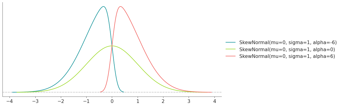
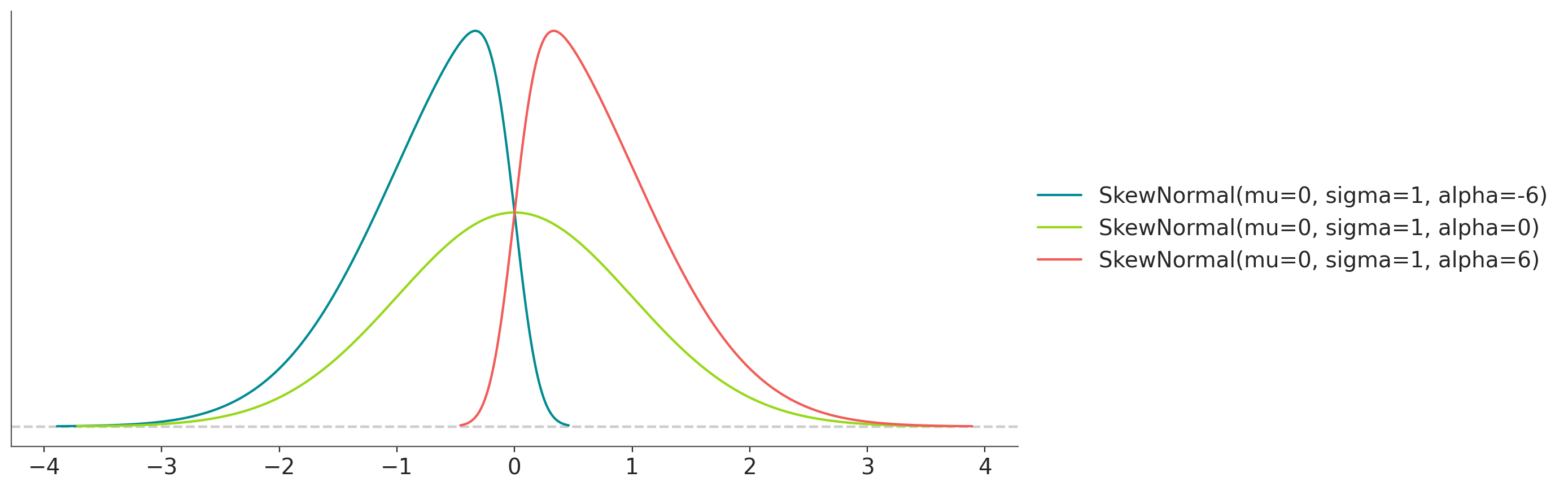
class preliz.distributions.skew_studentt.SkewStudentT(mu=None, sigma=None, a=None, b=None, lam=None)[source]#

Jones and Faddy’s Skewed Student-t distribution.

The pdf of this distribution is

\[f(t)=f(t ; a, b)=C_{a, b}^{-1}\left\{1+\frac{t}{\left(a+b+t^2\right)^{1 / 2}} \right\}^{a+1 / 2}\left\{1-\frac{t}{\left(a+b+t^2\right)^{1 / 2}}\right\}^{b+1 / 2}\]

where

\[C_{a, b}=2^{a+b-1} B(a, b)(a+b)^{1 / 2}\]

(Source code, png, hires.png, pdf)

Support	$x \in \mathbb{R}$
Mean	\[\mu + \sigma\frac{(a-b) \sqrt{(a+b)}}{2}\frac{\Gamma\left(a-\frac{1}{2}\right) \Gamma\left(b-\frac{1}{2}\right)}{\Gamma(a) \Gamma(b)}\]

Parameters:

mu (float) – Location Parameter
sigma (float) – Scale parameter (sigma > 0). Converges to the standard deviation as a and b approach close
a (float) – First Shape Parameter (a > 0)
b (float) – Second Shape Parameter (b > 0)
lam (float) – Scale Parameter (lam > 0). Converges to the precision as a and b approach close

Notes

If a > b, the distribution is positively skewed, and if a < b, the distribution is negatively skewed. If a = b, the distribution is StudentT with nu (degrees of freedom) = 2a.

cdf(x)[source]#

Cumulative distribution function.

Parameters:: x (array_like) – Values on which to evaluate the cdf

entropy()[source]#: Entropy.

eti(mass=None, fmt='.2f')#

Equal-tailed interval containing mass.

Parameters:

mass (float) – Probability mass in the interval. Defaults to None,
used. (which results in the value of rcParams["stats.ci_prob"] being)
fmt (str) – fmt used to represent results using f-string fmt for floats. Default to “.2f” i.e. 2 digits after the decimal point. Use “none” for no format.

hdi(mass=None, fmt='.2f')#

Highest density interval containing mass.

Parameters:

mass (float) – Probability mass in the interval. Defaults to None,
used. (which results in the value of rcParams["stats.ci_prob"] being)
fmt (str) – fmt used to represent results using f-string fmt for floats. Default to “.2f” i.e. 2 digits after the decimal point. Use “none” for no format.

isf(x)#

Inverse survival function (inverse of sf).

Parameters:: x (array_like) – Values on which to evaluate the inverse of the sf

kurtosis()[source]#: Excess kurtosis.

lmoment1()[source]#: L-moment1 (mean).

lmoment2()[source]#: L-moment2 (l-scale).

lmoment3()[source]#: L-moment3 (l-skewness). This the ratio of L-moment3 to L-moment2.

lmoment4()[source]#: L-moment4 (l-kurtosis). This the ratio of L-moment4 to L-moment2.

lmoments(types='1234')#

Compute L-moments of the distribution.

Parameters:: types (str) – The type of moments to compute. Default is ‘1234’ where ‘1’ = L-moment1 (mean), ‘2’ = L-moment2 (l-scale), ‘3’ = L-moment3 (l-skewness), and ‘4’ = L-moment4 (l-kurtosis). To compute the standard deviation use ‘d’ Valid combinations are any subset of ‘1234’.

logcdf(x)#

Log cumulative distribution function.

Parameters:: x (array_like) – Values on which to evaluate the logcdf

logpdf(x)[source]#

Log probability density/mass function.

Parameters:: x (array_like) – Values on which to evaluate the logpdf

logsf(x)#

Log survival function log(1 - cdf).

Parameters:: x (array_like) – Values on which to evaluate the logsf

mean()[source]#: Mean.

median()[source]#: Median.

mode()#: Mode.

moments(types='mvsk')#

Compute moments of the distribution.

It can also return the standard deviation

Parameters:: types (str) – The type of moments to compute. Default is ‘mvsk’ where ‘m’ = mean, ‘v’ = variance, ‘s’ = skewness, and ‘k’ = kurtosis. To compute the standard deviation use ‘d’ Valid combinations are any subset of ‘mvdsk’.

pdf(x)[source]#

Probability density/mass function.

Parameters:: x (array_like) – Values on which to evaluate the pdf

plot_cdf(moments=None, pointinterval=False, interval=None, levels=None, support='restricted', legend='legend', figsize=None, ax=None, **kwargs)#

Plot the cumulative distribution function.

Parameters:

moments (str) – Compute moments. Use any combination of the strings m, d, v, s or k for the mean (μ), standard deviation (σ), variance (σ²), skew (γ) or kurtosis (κ) respectively. Other strings will be ignored. Defaults to None.
pointinterval (bool) – Whether to include a plot of the quantiles. Defaults to False. If True the default is to plot the median and two interquantiles ranges.
interval (str) – Type of interval. Available options are highest density interval “hdi” (default), equal tailed interval “eti” or intervals defined by arbitrary “quantiles”. Defaults to the value in rcParams[“stats.ci_kind”].
levels (list) – Mass of the intervals. For hdi or eti the number of elements should be 2 or 1. For quantiles the number of elements should be 5, 3, 1 or 0 (in this last case nothing will be plotted).
support (str:) – If full use the finite end-points to set the limits of the plot. For unbounded end-points or if restricted use the 0.001 and 0.999 quantiles to set the limits.
legend (str) – Whether to include a string with the distribution and its parameter as a "legend" a "title" or not include them None.
figsize (tuple) – Size of the figure
ax (matplotlib axes)
kwargs (keyword arguments) – Additional keyword arguments passed to matplotlib plot function. For example, color, alpha, linewidth, etc.

plot_interactive(kind='pdf', xy_lim='both', pointinterval=True, interval=None, levels=None, figsize=None)#

Interactive exploration of distributions parameters.

Parameters:

kind (str:) – Type of plot. Available options are pdf, cdf and ppf.
xy_lim (str or tuple) – Set the limits of the x-axis and/or y-axis. Defaults to “both”, the limits of both axis are fixed. Use “auto” for automatic rescaling of x-axis and y-axis. Or set them manually by passing a tuple of 4 elements, the first two for x-axis, the last two for y-axis. The tuple can have None.
pointinterval (bool) – Whether to include a plot of the quantiles. Defaults to False. If True the default is to plot the median and two interquantiles ranges.
interval (str) – Type of interval. Available options are highest density interval “hdi” (default), equal tailed interval “eti” or intervals defined by arbitrary “quantiles”. Defaults to the value in rcParams[“stats.ci_kind”].
levels (list) – Mass of the intervals. For hdi or eti the number of elements should be 2 or 1. For quantiles the number of elements should be 5, 3, 1 or 0 (in this last case nothing will be plotted).
figsize (tuple) – Size of the figure

plot_isf(moments=None, pointinterval=False, interval=None, levels=None, legend='legend', figsize=None, ax=None, **kwargs)#

Plot the inverse survival function.

Parameters:

moments (str) – Compute moments. Use any combination of the strings m, d, v, s or k for the mean (μ), standard deviation (σ), variance (σ²), skew (γ) or kurtosis (κ) respectively. Other strings will be ignored. Defaults to None.
pointinterval (bool) – Whether to include a plot of the quantiles. Defaults to False. If True the default is to plot the median and two interquantiles ranges.
interval (str) – Type of interval. Available options are highest density interval “hdi” (default), equal tailed interval “eti” or intervals defined by arbitrary “quantiles”. Defaults to the value in rcParams[“stats.ci_kind”].
levels (list) – Mass of the intervals. For hdi or eti the number of elements should be 2 or 1. For quantiles the number of elements should be 5, 3, 1 or 0 (in this last case nothing will be plotted).
legend (str) – Whether to include a string with the distribution and its parameter as a "legend" a "title" or not include them None.
figsize (tuple) – Size of the figure
ax (matplotlib axes)

plot_pdf(moments=None, pointinterval=False, interval=None, levels=None, support='restricted', baseline=True, legend='legend', figsize=None, ax=None, **kwargs)#

Plot the pdf (continuous) or pmf (discrete).

Parameters:

moments (str) – Compute moments. Use any combination of the strings m, d, v, s or k for the mean (μ), standard deviation (σ), variance (σ²), skew (γ) or kurtosis (κ) respectively. Other strings will be ignored. Defaults to None.
pointinterval (bool) – Whether to include a plot of the quantiles. Defaults to False. If True the default is to plot the median and two interquantiles ranges.
interval (str) – Type of interval. Available options are highest density interval “hdi” (default), equal tailed interval “eti” or intervals defined by arbitrary “quantiles”. Defaults to the value in rcParams[“stats.ci_kind”].
levels (list) – Mass of the intervals. For hdi or eti the number of elements should be 2 or 1. For quantiles the number of elements should be 5, 3, 1 or 0 (in this last case nothing will be plotted).
support (str:) – If full use the finite end-points to set the limits of the plot. For unbounded end-points or if restricted use the 0.001 and 0.999 quantiles to set the limits.
baseline (bool) – Whether to include a horizontal line at y=0.
legend (str) – Whether to include a string with the distribution and its parameter as a "legend" a "title" or not include them None.
figsize (tuple) – Size of the figure
ax (matplotlib axes)
kwargs (keyword arguments) – Additional keyword arguments passed to matplotlib plot function. For example, color, alpha, linewidth, etc.

plot_ppf(moments=None, pointinterval=False, interval=None, levels=None, legend='legend', figsize=None, ax=None, **kwargs)#

Plot the quantile function.

Parameters:

moments (str) – Compute moments. Use any combination of the strings m, d, v, s or k for the mean (μ), standard deviation (σ), variance (σ²), skew (γ) or kurtosis (κ) respectively. Other strings will be ignored. Defaults to None.
pointinterval (bool) – Whether to include a plot of the quantiles. Defaults to False. If True the default is to plot the median and two interquantiles ranges.
interval (str) – Type of interval. Available options are highest density interval “hdi” (default), equal tailed interval “eti” or intervals defined by arbitrary “quantiles”. Defaults to the value in rcParams[“stats.ci_kind”].
levels (list) – Mass of the intervals. For hdi or eti the number of elements should be 2 or 1. For quantiles the number of elements should be 5, 3, 1 or 0 (in this last case nothing will be plotted).
legend (str) – Whether to include a string with the distribution and its parameter as a "legend" a "title" or not include them None.
figsize (tuple) – Size of the figure
ax (matplotlib axes)

plot_sf(moments=None, pointinterval=False, interval=None, levels=None, support='restricted', legend='legend', figsize=None, ax=None, **kwargs)#

Plot the survival distribution function (1 - CDF).

Parameters:

moments (str) – Compute moments. Use any combination of the strings m, d, v, s or k for the mean (μ), standard deviation (σ), variance (σ²), skew (γ) or kurtosis (κ) respectively. Other strings will be ignored. Defaults to None.
pointinterval (bool) – Whether to include a plot of the quantiles. Defaults to False. If True the default is to plot the median and two interquantiles ranges.
interval (str) – Type of interval. Available options are highest density interval “hdi” (default), equal tailed interval “eti” or intervals defined by arbitrary “quantiles”. Defaults to the value in rcParams[“stats.ci_kind”].
levels (list) – Mass of the intervals. For hdi or eti the number of elements should be 2 or 1. For quantiles the number of elements should be 5, 3, 1 or 0 (in this last case nothing will be plotted).
support (str:) – If full use the finite end-points to set the limits of the plot. For unbounded end-points or if restricted use the 0.001 and 0.999 quantiles to set the limits.
legend (str) – Whether to include a string with the distribution and its parameter as a "legend" a "title" or not include them None.
figsize (tuple) – Size of the figure
ax (matplotlib axes)
kwargs (keyword arguments) – Additional keyword arguments passed to matplotlib plot function. For example, color, alpha, linewidth, etc.

ppf(q)[source]#

Percent point function (inverse of cdf).

Parameters:: x (array_like) – Values on which to evaluate the inverse of the cdf

rvs(size=None, random_state=None)[source]#

Random sample.

Parameters:

size (int or tuple of ints, optional) – Defining number of random variates. Defaults to 1.
random_state ({None, int, numpy.random.Generator, numpy.random.RandomState}) – Defaults to None

sf(x)#

Survival function (1 - cdf).

Parameters:: x (array_like) – Values on which to evaluate the sf

skewness()[source]#: Skewness.

std()[source]#: Standard deviation.

summary(mass=None, interval=None, fmt='.2f')#

Namedtuple with the mean, median, sd, and lower and upper bounds.

Parameters:

mass (float) – Probability mass for the equal-tailed interval. Defaults to None,
used. (which results in the value of rcParams["stats.ci_prob"] being)
interval (str or list-like) – Type of interval. Available options are highest density interval “hdi”, equal tailed interval “eti” or arbitrary interval defined by a list-like object with a pair of values. Defaults to the value in rcParams[“stats.ci_kind”].
fmt (str) – fmt used to represent results using f-string fmt for floats. Default to “.2f” i.e. 2 digits after the decimal point.

to_bambi(**kwargs)#

Convert the PreliZ distribution to a Bambi Prior.

kwargsPyMC distributions properties: kwargs are used to specify properties such as shape or dims

Return type:: Bambi Prior

to_pymc(name=None, **kwargs)#

Convert the PreliZ distribution to a PyMC distribution.

namestr: Name of PyMC distribution. Needed if inside Model context
kwargsPyMC distributions properties: kwargs are used to specify properties such as shape or dims

Return type:: PyMC distribution

var()[source]#: Variance.

xvals(support, n_points=None)#

Provide x values in the support of the distribution.

This is useful for example when plotting.

Parameters:

support (str) – Available options are “full” or “restricted”. If “full” the values will cover the entire support of the distribution if the boundary is finite, or the quantiles 0.0001 or 0.9999, if infinite. If “restricted” the values will cover the quantile 0.0001 to 0.9999.
n_points (int) – Number of values to return. Defaults to 1000 for continuous distributions and 200 for discrete ones. For discrete distributions the returned values may be fewer than n_points if the actual number of discrete values in the support of the distribution is smaller than n_points.

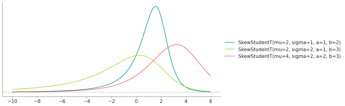
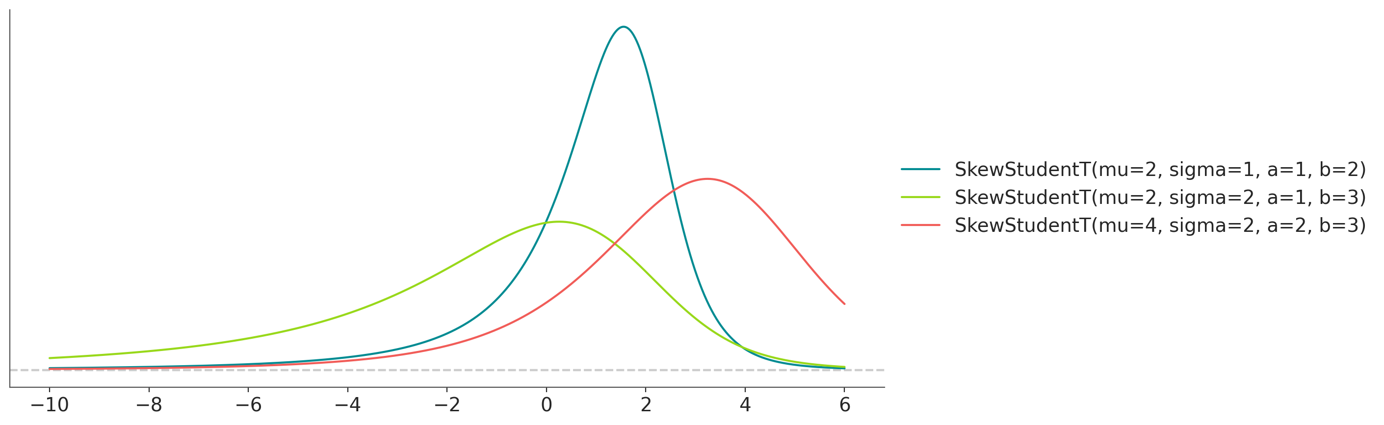
class preliz.distributions.studentt.StudentT(nu=None, mu=None, sigma=None, lam=None)[source]#

StudentT’s distribution.

Describes a normal variable whose precision is gamma distributed.

The pdf of this distribution is

\[f(x \mid \nu, \mu, \sigma) = \frac{\Gamma \left(\frac{\nu+1}{2} \right)} {\sqrt{\nu\pi}\ \Gamma \left(\frac{\nu}{2} \right)} \left(1+\frac{x^2}{\nu} \right)^{-\frac{\nu+1}{2}}\]

(Source code, png, hires.png, pdf)

Support	$x \in \mathbb{R}$
Mean	$\mu$ for $\nu > 1$, otherwise undefined
Variance	$\frac{\nu}{\nu-2}$ for $\nu > 2$, $\infty$ for $1 < \nu \le 2$, otherwise undefined

StudentT distribution has 2 alternative parameterization. In terms of nu, mu and sigma (standard deviation as nu increases) or nu, mu and lam (precision as nu increases).

The link between the 2 alternatives is given by

\[\lambda = \frac{1}{\sigma^2}\]

Parameters:

nu (float) – Degrees of freedom, also known as normality parameter (nu > 0).
mu (float) – Location parameter.
sigma (float) – Scale parameter (sigma > 0). Converges to the standard deviation as nu increases.
lam (float) – Scale parameter (lam > 0). Converges to the precision as nu increases.

cdf(x)[source]#

Cumulative distribution function.

Parameters:: x (array_like) – Values on which to evaluate the cdf

entropy()[source]#: Entropy.

eti(mass=None, fmt='.2f')#

Equal-tailed interval containing mass.

Parameters:

mass (float) – Probability mass in the interval. Defaults to None,
used. (which results in the value of rcParams["stats.ci_prob"] being)
fmt (str) – fmt used to represent results using f-string fmt for floats. Default to “.2f” i.e. 2 digits after the decimal point. Use “none” for no format.

hdi(mass=None, fmt='.2f')#

Highest density interval containing mass.

Parameters:

mass (float) – Probability mass in the interval. Defaults to None,
used. (which results in the value of rcParams["stats.ci_prob"] being)
fmt (str) – fmt used to represent results using f-string fmt for floats. Default to “.2f” i.e. 2 digits after the decimal point. Use “none” for no format.

isf(x)#

Inverse survival function (inverse of sf).

Parameters:: x (array_like) – Values on which to evaluate the inverse of the sf

kurtosis()[source]#: Excess kurtosis.

lmoment1()[source]#: L-moment1 (mean).

lmoment2()[source]#: L-moment2 (l-scale).

lmoment3()[source]#: L-moment3 (l-skewness). This the ratio of L-moment3 to L-moment2.

lmoment4()[source]#: L-moment4 (l-kurtosis). This the ratio of L-moment4 to L-moment2.

lmoments(types='1234')#

Compute L-moments of the distribution.

Parameters:: types (str) – The type of moments to compute. Default is ‘1234’ where ‘1’ = L-moment1 (mean), ‘2’ = L-moment2 (l-scale), ‘3’ = L-moment3 (l-skewness), and ‘4’ = L-moment4 (l-kurtosis). To compute the standard deviation use ‘d’ Valid combinations are any subset of ‘1234’.

logcdf(x)#

Log cumulative distribution function.

Parameters:: x (array_like) – Values on which to evaluate the logcdf

logpdf(x)[source]#

Log probability density/mass function.

Parameters:: x (array_like) – Values on which to evaluate the logpdf

logsf(x)#

Log survival function log(1 - cdf).

Parameters:: x (array_like) – Values on which to evaluate the logsf

mean()[source]#: Mean.

median()[source]#: Median.

mode()[source]#: Mode.

moments(types='mvsk')#

Compute moments of the distribution.

It can also return the standard deviation

Parameters:: types (str) – The type of moments to compute. Default is ‘mvsk’ where ‘m’ = mean, ‘v’ = variance, ‘s’ = skewness, and ‘k’ = kurtosis. To compute the standard deviation use ‘d’ Valid combinations are any subset of ‘mvdsk’.

pdf(x)[source]#

Probability density/mass function.

Parameters:: x (array_like) – Values on which to evaluate the pdf

plot_cdf(moments=None, pointinterval=False, interval=None, levels=None, support='restricted', legend='legend', figsize=None, ax=None, **kwargs)#

Plot the cumulative distribution function.

Parameters:

moments (str) – Compute moments. Use any combination of the strings m, d, v, s or k for the mean (μ), standard deviation (σ), variance (σ²), skew (γ) or kurtosis (κ) respectively. Other strings will be ignored. Defaults to None.
pointinterval (bool) – Whether to include a plot of the quantiles. Defaults to False. If True the default is to plot the median and two interquantiles ranges.
interval (str) – Type of interval. Available options are highest density interval “hdi” (default), equal tailed interval “eti” or intervals defined by arbitrary “quantiles”. Defaults to the value in rcParams[“stats.ci_kind”].
levels (list) – Mass of the intervals. For hdi or eti the number of elements should be 2 or 1. For quantiles the number of elements should be 5, 3, 1 or 0 (in this last case nothing will be plotted).
support (str:) – If full use the finite end-points to set the limits of the plot. For unbounded end-points or if restricted use the 0.001 and 0.999 quantiles to set the limits.
legend (str) – Whether to include a string with the distribution and its parameter as a "legend" a "title" or not include them None.
figsize (tuple) – Size of the figure
ax (matplotlib axes)
kwargs (keyword arguments) – Additional keyword arguments passed to matplotlib plot function. For example, color, alpha, linewidth, etc.

plot_interactive(kind='pdf', xy_lim='both', pointinterval=True, interval=None, levels=None, figsize=None)#

Interactive exploration of distributions parameters.

Parameters:

kind (str:) – Type of plot. Available options are pdf, cdf and ppf.
xy_lim (str or tuple) – Set the limits of the x-axis and/or y-axis. Defaults to “both”, the limits of both axis are fixed. Use “auto” for automatic rescaling of x-axis and y-axis. Or set them manually by passing a tuple of 4 elements, the first two for x-axis, the last two for y-axis. The tuple can have None.
pointinterval (bool) – Whether to include a plot of the quantiles. Defaults to False. If True the default is to plot the median and two interquantiles ranges.
interval (str) – Type of interval. Available options are highest density interval “hdi” (default), equal tailed interval “eti” or intervals defined by arbitrary “quantiles”. Defaults to the value in rcParams[“stats.ci_kind”].
levels (list) – Mass of the intervals. For hdi or eti the number of elements should be 2 or 1. For quantiles the number of elements should be 5, 3, 1 or 0 (in this last case nothing will be plotted).
figsize (tuple) – Size of the figure

plot_isf(moments=None, pointinterval=False, interval=None, levels=None, legend='legend', figsize=None, ax=None, **kwargs)#

Plot the inverse survival function.

Parameters:

moments (str) – Compute moments. Use any combination of the strings m, d, v, s or k for the mean (μ), standard deviation (σ), variance (σ²), skew (γ) or kurtosis (κ) respectively. Other strings will be ignored. Defaults to None.
pointinterval (bool) – Whether to include a plot of the quantiles. Defaults to False. If True the default is to plot the median and two interquantiles ranges.
interval (str) – Type of interval. Available options are highest density interval “hdi” (default), equal tailed interval “eti” or intervals defined by arbitrary “quantiles”. Defaults to the value in rcParams[“stats.ci_kind”].
levels (list) – Mass of the intervals. For hdi or eti the number of elements should be 2 or 1. For quantiles the number of elements should be 5, 3, 1 or 0 (in this last case nothing will be plotted).
legend (str) – Whether to include a string with the distribution and its parameter as a "legend" a "title" or not include them None.
figsize (tuple) – Size of the figure
ax (matplotlib axes)

plot_pdf(moments=None, pointinterval=False, interval=None, levels=None, support='restricted', baseline=True, legend='legend', figsize=None, ax=None, **kwargs)#

Plot the pdf (continuous) or pmf (discrete).

Parameters:

moments (str) – Compute moments. Use any combination of the strings m, d, v, s or k for the mean (μ), standard deviation (σ), variance (σ²), skew (γ) or kurtosis (κ) respectively. Other strings will be ignored. Defaults to None.
pointinterval (bool) – Whether to include a plot of the quantiles. Defaults to False. If True the default is to plot the median and two interquantiles ranges.
interval (str) – Type of interval. Available options are highest density interval “hdi” (default), equal tailed interval “eti” or intervals defined by arbitrary “quantiles”. Defaults to the value in rcParams[“stats.ci_kind”].
levels (list) – Mass of the intervals. For hdi or eti the number of elements should be 2 or 1. For quantiles the number of elements should be 5, 3, 1 or 0 (in this last case nothing will be plotted).
support (str:) – If full use the finite end-points to set the limits of the plot. For unbounded end-points or if restricted use the 0.001 and 0.999 quantiles to set the limits.
baseline (bool) – Whether to include a horizontal line at y=0.
legend (str) – Whether to include a string with the distribution and its parameter as a "legend" a "title" or not include them None.
figsize (tuple) – Size of the figure
ax (matplotlib axes)
kwargs (keyword arguments) – Additional keyword arguments passed to matplotlib plot function. For example, color, alpha, linewidth, etc.

plot_ppf(moments=None, pointinterval=False, interval=None, levels=None, legend='legend', figsize=None, ax=None, **kwargs)#

Plot the quantile function.

Parameters:

moments (str) – Compute moments. Use any combination of the strings m, d, v, s or k for the mean (μ), standard deviation (σ), variance (σ²), skew (γ) or kurtosis (κ) respectively. Other strings will be ignored. Defaults to None.
pointinterval (bool) – Whether to include a plot of the quantiles. Defaults to False. If True the default is to plot the median and two interquantiles ranges.
interval (str) – Type of interval. Available options are highest density interval “hdi” (default), equal tailed interval “eti” or intervals defined by arbitrary “quantiles”. Defaults to the value in rcParams[“stats.ci_kind”].
levels (list) – Mass of the intervals. For hdi or eti the number of elements should be 2 or 1. For quantiles the number of elements should be 5, 3, 1 or 0 (in this last case nothing will be plotted).
legend (str) – Whether to include a string with the distribution and its parameter as a "legend" a "title" or not include them None.
figsize (tuple) – Size of the figure
ax (matplotlib axes)

plot_sf(moments=None, pointinterval=False, interval=None, levels=None, support='restricted', legend='legend', figsize=None, ax=None, **kwargs)#

Plot the survival distribution function (1 - CDF).

Parameters:

moments (str) – Compute moments. Use any combination of the strings m, d, v, s or k for the mean (μ), standard deviation (σ), variance (σ²), skew (γ) or kurtosis (κ) respectively. Other strings will be ignored. Defaults to None.
pointinterval (bool) – Whether to include a plot of the quantiles. Defaults to False. If True the default is to plot the median and two interquantiles ranges.
interval (str) – Type of interval. Available options are highest density interval “hdi” (default), equal tailed interval “eti” or intervals defined by arbitrary “quantiles”. Defaults to the value in rcParams[“stats.ci_kind”].
levels (list) – Mass of the intervals. For hdi or eti the number of elements should be 2 or 1. For quantiles the number of elements should be 5, 3, 1 or 0 (in this last case nothing will be plotted).
support (str:) – If full use the finite end-points to set the limits of the plot. For unbounded end-points or if restricted use the 0.001 and 0.999 quantiles to set the limits.
legend (str) – Whether to include a string with the distribution and its parameter as a "legend" a "title" or not include them None.
figsize (tuple) – Size of the figure
ax (matplotlib axes)
kwargs (keyword arguments) – Additional keyword arguments passed to matplotlib plot function. For example, color, alpha, linewidth, etc.

ppf(q)[source]#

Percent point function (inverse of cdf).

Parameters:: x (array_like) – Values on which to evaluate the inverse of the cdf

rvs(size=None, random_state=None)[source]#

Random sample.

Parameters:

size (int or tuple of ints, optional) – Defining number of random variates. Defaults to 1.
random_state ({None, int, numpy.random.Generator, numpy.random.RandomState}) – Defaults to None

sf(x)#

Survival function (1 - cdf).

Parameters:: x (array_like) – Values on which to evaluate the sf

skewness()[source]#: Skewness.

std()[source]#: Standard deviation.

summary(mass=None, interval=None, fmt='.2f')#

Namedtuple with the mean, median, sd, and lower and upper bounds.

Parameters:

mass (float) – Probability mass for the equal-tailed interval. Defaults to None,
used. (which results in the value of rcParams["stats.ci_prob"] being)
interval (str or list-like) – Type of interval. Available options are highest density interval “hdi”, equal tailed interval “eti” or arbitrary interval defined by a list-like object with a pair of values. Defaults to the value in rcParams[“stats.ci_kind”].
fmt (str) – fmt used to represent results using f-string fmt for floats. Default to “.2f” i.e. 2 digits after the decimal point.

to_bambi(**kwargs)#

Convert the PreliZ distribution to a Bambi Prior.

kwargsPyMC distributions properties: kwargs are used to specify properties such as shape or dims

Return type:: Bambi Prior

to_pymc(name=None, **kwargs)#

Convert the PreliZ distribution to a PyMC distribution.

namestr: Name of PyMC distribution. Needed if inside Model context
kwargsPyMC distributions properties: kwargs are used to specify properties such as shape or dims

Return type:: PyMC distribution

var()[source]#: Variance.

xvals(support, n_points=None)#

Provide x values in the support of the distribution.

This is useful for example when plotting.

Parameters:

support (str) – Available options are “full” or “restricted”. If “full” the values will cover the entire support of the distribution if the boundary is finite, or the quantiles 0.0001 or 0.9999, if infinite. If “restricted” the values will cover the quantile 0.0001 to 0.9999.
n_points (int) – Number of values to return. Defaults to 1000 for continuous distributions and 200 for discrete ones. For discrete distributions the returned values may be fewer than n_points if the actual number of discrete values in the support of the distribution is smaller than n_points.

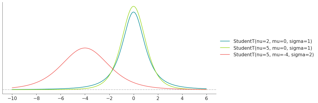
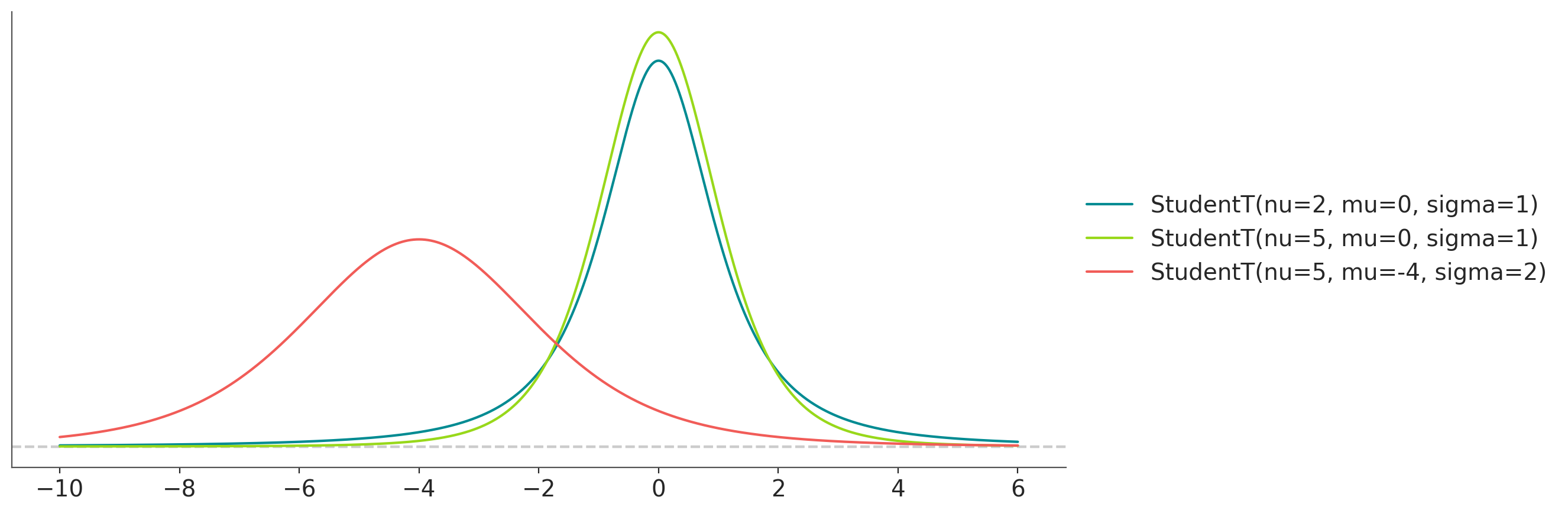
class preliz.distributions.triangular.Triangular(lower=None, c=None, upper=None)[source]#

Triangular distribution.

The pdf of this distribution is

\[\begin{split}\begin{cases} 0 & \text{for } x < a, \\ \frac{2(x-a)}{(b-a)(c-a)} & \text{for } a \le x < c, \\[4pt] \frac{2}{b-a} & \text{for } x = c, \\[4pt] \frac{2(b-x)}{(b-a)(b-c)} & \text{for } c < x \le b, \\[4pt] 0 & \text{for } b < x. \end{cases}\end{split}\]

(Source code, png, hires.png, pdf)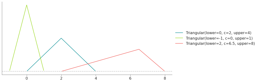

Support	$x \in [lower, upper]$
Mean	$\dfrac{lower + upper + c}{3}$
Variance	$\dfrac{upper^2 + lower^2 +c^2 - lowerupper - lowerc - upper*c}{18}$

Parameters:

lower (float) – Lower limit.
c (float) – Mode.
upper (float) – Upper limit.

cdf(x)[source]#

Cumulative distribution function.

Parameters:: x (array_like) – Values on which to evaluate the cdf

entropy()[source]#: Entropy.

eti(mass=None, fmt='.2f')#

Equal-tailed interval containing mass.

Parameters:

mass (float) – Probability mass in the interval. Defaults to None,
used. (which results in the value of rcParams["stats.ci_prob"] being)
fmt (str) – fmt used to represent results using f-string fmt for floats. Default to “.2f” i.e. 2 digits after the decimal point. Use “none” for no format.

hdi(mass=None, fmt='.2f')#

Highest density interval containing mass.

Parameters:

mass (float) – Probability mass in the interval. Defaults to None,
used. (which results in the value of rcParams["stats.ci_prob"] being)
fmt (str) – fmt used to represent results using f-string fmt for floats. Default to “.2f” i.e. 2 digits after the decimal point. Use “none” for no format.

isf(x)#

Inverse survival function (inverse of sf).

Parameters:: x (array_like) – Values on which to evaluate the inverse of the sf

kurtosis()[source]#: Excess kurtosis.

lmoment1()[source]#: L-moment1 (mean).

lmoment2()[source]#: L-moment2 (l-scale).

lmoment3()[source]#: L-moment3 (l-skewness). This the ratio of L-moment3 to L-moment2.

lmoment4()[source]#: L-moment4 (l-kurtosis). This the ratio of L-moment4 to L-moment2.

lmoments(types='1234')#

Compute L-moments of the distribution.

Parameters:: types (str) – The type of moments to compute. Default is ‘1234’ where ‘1’ = L-moment1 (mean), ‘2’ = L-moment2 (l-scale), ‘3’ = L-moment3 (l-skewness), and ‘4’ = L-moment4 (l-kurtosis). To compute the standard deviation use ‘d’ Valid combinations are any subset of ‘1234’.

logcdf(x)#

Log cumulative distribution function.

Parameters:: x (array_like) – Values on which to evaluate the logcdf

logpdf(x)[source]#

Log probability density/mass function.

Parameters:: x (array_like) – Values on which to evaluate the logpdf

logsf(x)#

Log survival function log(1 - cdf).

Parameters:: x (array_like) – Values on which to evaluate the logsf

mean()[source]#: Mean.

median()[source]#: Median.

mode()[source]#: Mode.

moments(types='mvsk')#

Compute moments of the distribution.

It can also return the standard deviation

Parameters:: types (str) – The type of moments to compute. Default is ‘mvsk’ where ‘m’ = mean, ‘v’ = variance, ‘s’ = skewness, and ‘k’ = kurtosis. To compute the standard deviation use ‘d’ Valid combinations are any subset of ‘mvdsk’.

pdf(x)[source]#

Probability density/mass function.

Parameters:: x (array_like) – Values on which to evaluate the pdf

plot_cdf(moments=None, pointinterval=False, interval=None, levels=None, support='restricted', legend='legend', figsize=None, ax=None, **kwargs)#

Plot the cumulative distribution function.

Parameters:

moments (str) – Compute moments. Use any combination of the strings m, d, v, s or k for the mean (μ), standard deviation (σ), variance (σ²), skew (γ) or kurtosis (κ) respectively. Other strings will be ignored. Defaults to None.
pointinterval (bool) – Whether to include a plot of the quantiles. Defaults to False. If True the default is to plot the median and two interquantiles ranges.
interval (str) – Type of interval. Available options are highest density interval “hdi” (default), equal tailed interval “eti” or intervals defined by arbitrary “quantiles”. Defaults to the value in rcParams[“stats.ci_kind”].
levels (list) – Mass of the intervals. For hdi or eti the number of elements should be 2 or 1. For quantiles the number of elements should be 5, 3, 1 or 0 (in this last case nothing will be plotted).
support (str:) – If full use the finite end-points to set the limits of the plot. For unbounded end-points or if restricted use the 0.001 and 0.999 quantiles to set the limits.
legend (str) – Whether to include a string with the distribution and its parameter as a "legend" a "title" or not include them None.
figsize (tuple) – Size of the figure
ax (matplotlib axes)
kwargs (keyword arguments) – Additional keyword arguments passed to matplotlib plot function. For example, color, alpha, linewidth, etc.

plot_interactive(kind='pdf', xy_lim='both', pointinterval=True, interval=None, levels=None, figsize=None)#

Interactive exploration of distributions parameters.

Parameters:

kind (str:) – Type of plot. Available options are pdf, cdf and ppf.
xy_lim (str or tuple) – Set the limits of the x-axis and/or y-axis. Defaults to “both”, the limits of both axis are fixed. Use “auto” for automatic rescaling of x-axis and y-axis. Or set them manually by passing a tuple of 4 elements, the first two for x-axis, the last two for y-axis. The tuple can have None.
pointinterval (bool) – Whether to include a plot of the quantiles. Defaults to False. If True the default is to plot the median and two interquantiles ranges.
interval (str) – Type of interval. Available options are highest density interval “hdi” (default), equal tailed interval “eti” or intervals defined by arbitrary “quantiles”. Defaults to the value in rcParams[“stats.ci_kind”].
levels (list) – Mass of the intervals. For hdi or eti the number of elements should be 2 or 1. For quantiles the number of elements should be 5, 3, 1 or 0 (in this last case nothing will be plotted).
figsize (tuple) – Size of the figure

plot_isf(moments=None, pointinterval=False, interval=None, levels=None, legend='legend', figsize=None, ax=None, **kwargs)#

Plot the inverse survival function.

Parameters:

moments (str) – Compute moments. Use any combination of the strings m, d, v, s or k for the mean (μ), standard deviation (σ), variance (σ²), skew (γ) or kurtosis (κ) respectively. Other strings will be ignored. Defaults to None.
pointinterval (bool) – Whether to include a plot of the quantiles. Defaults to False. If True the default is to plot the median and two interquantiles ranges.
interval (str) – Type of interval. Available options are highest density interval “hdi” (default), equal tailed interval “eti” or intervals defined by arbitrary “quantiles”. Defaults to the value in rcParams[“stats.ci_kind”].
levels (list) – Mass of the intervals. For hdi or eti the number of elements should be 2 or 1. For quantiles the number of elements should be 5, 3, 1 or 0 (in this last case nothing will be plotted).
legend (str) – Whether to include a string with the distribution and its parameter as a "legend" a "title" or not include them None.
figsize (tuple) – Size of the figure
ax (matplotlib axes)

plot_pdf(moments=None, pointinterval=False, interval=None, levels=None, support='restricted', baseline=True, legend='legend', figsize=None, ax=None, **kwargs)#

Plot the pdf (continuous) or pmf (discrete).

Parameters:

moments (str) – Compute moments. Use any combination of the strings m, d, v, s or k for the mean (μ), standard deviation (σ), variance (σ²), skew (γ) or kurtosis (κ) respectively. Other strings will be ignored. Defaults to None.
pointinterval (bool) – Whether to include a plot of the quantiles. Defaults to False. If True the default is to plot the median and two interquantiles ranges.
interval (str) – Type of interval. Available options are highest density interval “hdi” (default), equal tailed interval “eti” or intervals defined by arbitrary “quantiles”. Defaults to the value in rcParams[“stats.ci_kind”].
levels (list) – Mass of the intervals. For hdi or eti the number of elements should be 2 or 1. For quantiles the number of elements should be 5, 3, 1 or 0 (in this last case nothing will be plotted).
support (str:) – If full use the finite end-points to set the limits of the plot. For unbounded end-points or if restricted use the 0.001 and 0.999 quantiles to set the limits.
baseline (bool) – Whether to include a horizontal line at y=0.
legend (str) – Whether to include a string with the distribution and its parameter as a "legend" a "title" or not include them None.
figsize (tuple) – Size of the figure
ax (matplotlib axes)
kwargs (keyword arguments) – Additional keyword arguments passed to matplotlib plot function. For example, color, alpha, linewidth, etc.

plot_ppf(moments=None, pointinterval=False, interval=None, levels=None, legend='legend', figsize=None, ax=None, **kwargs)#

Plot the quantile function.

Parameters:

moments (str) – Compute moments. Use any combination of the strings m, d, v, s or k for the mean (μ), standard deviation (σ), variance (σ²), skew (γ) or kurtosis (κ) respectively. Other strings will be ignored. Defaults to None.
pointinterval (bool) – Whether to include a plot of the quantiles. Defaults to False. If True the default is to plot the median and two interquantiles ranges.
interval (str) – Type of interval. Available options are highest density interval “hdi” (default), equal tailed interval “eti” or intervals defined by arbitrary “quantiles”. Defaults to the value in rcParams[“stats.ci_kind”].
levels (list) – Mass of the intervals. For hdi or eti the number of elements should be 2 or 1. For quantiles the number of elements should be 5, 3, 1 or 0 (in this last case nothing will be plotted).
legend (str) – Whether to include a string with the distribution and its parameter as a "legend" a "title" or not include them None.
figsize (tuple) – Size of the figure
ax (matplotlib axes)

plot_sf(moments=None, pointinterval=False, interval=None, levels=None, support='restricted', legend='legend', figsize=None, ax=None, **kwargs)#

Plot the survival distribution function (1 - CDF).

Parameters:

moments (str) – Compute moments. Use any combination of the strings m, d, v, s or k for the mean (μ), standard deviation (σ), variance (σ²), skew (γ) or kurtosis (κ) respectively. Other strings will be ignored. Defaults to None.
pointinterval (bool) – Whether to include a plot of the quantiles. Defaults to False. If True the default is to plot the median and two interquantiles ranges.
interval (str) – Type of interval. Available options are highest density interval “hdi” (default), equal tailed interval “eti” or intervals defined by arbitrary “quantiles”. Defaults to the value in rcParams[“stats.ci_kind”].
levels (list) – Mass of the intervals. For hdi or eti the number of elements should be 2 or 1. For quantiles the number of elements should be 5, 3, 1 or 0 (in this last case nothing will be plotted).
support (str:) – If full use the finite end-points to set the limits of the plot. For unbounded end-points or if restricted use the 0.001 and 0.999 quantiles to set the limits.
legend (str) – Whether to include a string with the distribution and its parameter as a "legend" a "title" or not include them None.
figsize (tuple) – Size of the figure
ax (matplotlib axes)
kwargs (keyword arguments) – Additional keyword arguments passed to matplotlib plot function. For example, color, alpha, linewidth, etc.

ppf(q)[source]#

Percent point function (inverse of cdf).

Parameters:: x (array_like) – Values on which to evaluate the inverse of the cdf

rvs(size=None, random_state=None)[source]#

Random sample.

Parameters:

size (int or tuple of ints, optional) – Defining number of random variates. Defaults to 1.
random_state ({None, int, numpy.random.Generator, numpy.random.RandomState}) – Defaults to None

sf(x)#

Survival function (1 - cdf).

Parameters:: x (array_like) – Values on which to evaluate the sf

skewness()[source]#: Skewness.

std()[source]#: Standard deviation.

summary(mass=None, interval=None, fmt='.2f')#

Namedtuple with the mean, median, sd, and lower and upper bounds.

Parameters:

mass (float) – Probability mass for the equal-tailed interval. Defaults to None,
used. (which results in the value of rcParams["stats.ci_prob"] being)
interval (str or list-like) – Type of interval. Available options are highest density interval “hdi”, equal tailed interval “eti” or arbitrary interval defined by a list-like object with a pair of values. Defaults to the value in rcParams[“stats.ci_kind”].
fmt (str) – fmt used to represent results using f-string fmt for floats. Default to “.2f” i.e. 2 digits after the decimal point.

to_bambi(**kwargs)#

Convert the PreliZ distribution to a Bambi Prior.

kwargsPyMC distributions properties: kwargs are used to specify properties such as shape or dims

Return type:: Bambi Prior

to_pymc(name=None, **kwargs)#

Convert the PreliZ distribution to a PyMC distribution.

namestr: Name of PyMC distribution. Needed if inside Model context
kwargsPyMC distributions properties: kwargs are used to specify properties such as shape or dims

Return type:: PyMC distribution

var()[source]#: Variance.

xvals(support, n_points=None)#

Provide x values in the support of the distribution.

This is useful for example when plotting.

Parameters:

support (str) – Available options are “full” or “restricted”. If “full” the values will cover the entire support of the distribution if the boundary is finite, or the quantiles 0.0001 or 0.9999, if infinite. If “restricted” the values will cover the quantile 0.0001 to 0.9999.
n_points (int) – Number of values to return. Defaults to 1000 for continuous distributions and 200 for discrete ones. For discrete distributions the returned values may be fewer than n_points if the actual number of discrete values in the support of the distribution is smaller than n_points.

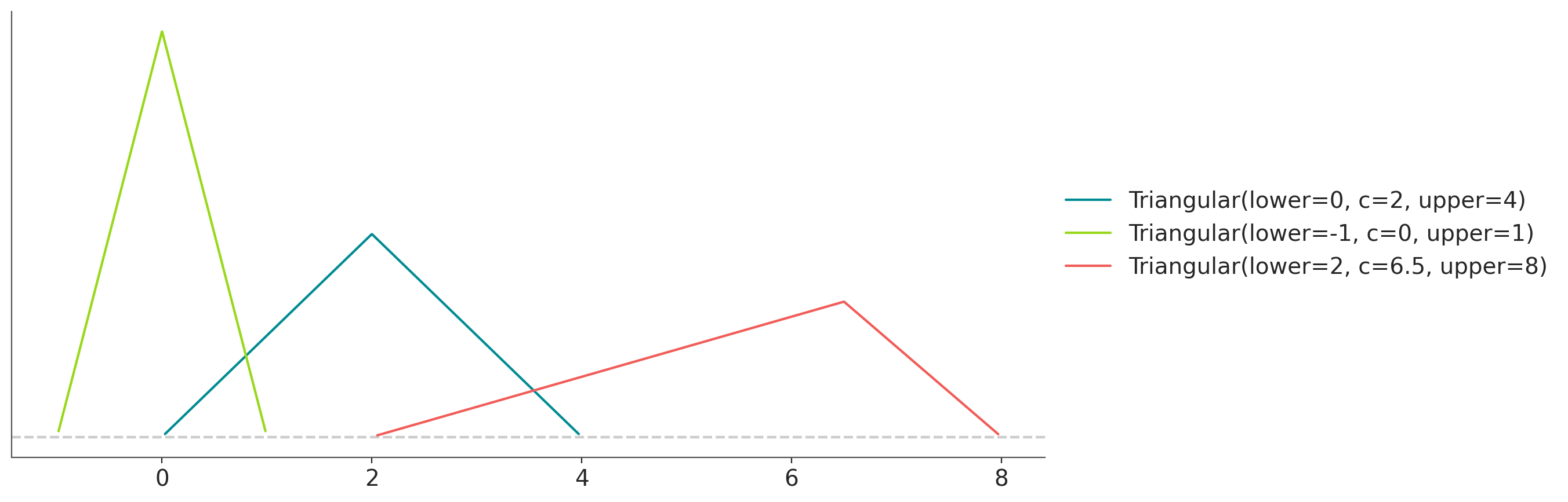
class preliz.distributions.truncatednormal.TruncatedNormal(mu=None, sigma=None, lower=None, upper=None)[source]#

TruncatedNormal distribution.

The pdf of this distribution is

\[f(x;\mu ,\sigma ,a,b)={\frac {\phi ({\frac {x-\mu }{\sigma }})}{ \sigma \left(\Phi ({\frac {b-\mu }{\sigma }})-\Phi ({\frac {a-\mu }{\sigma }})\right)}}\]

(Source code, png, hires.png, pdf)

Support	$x \in [a, b]$
Mean	$\mu +{\frac {\phi (\alpha )-\phi (\beta )}{Z}}\sigma$
Variance	\[\sigma ^{2}\left[1+{\frac {\alpha \phi (\alpha )-\beta \phi (\beta )}{Z}}- \left({\frac {\phi (\alpha )-\phi (\beta )}{Z}}\right)^{2}\right]\]

Parameters:

mu (float) – Mean.
sigma (float) – Standard deviation (sigma > 0)
lower (float) – Lower limit.
upper (float) – Upper limit (upper > lower).

cdf(x)[source]#

Cumulative distribution function.

Parameters:: x (array_like) – Values on which to evaluate the cdf

entropy()[source]#: Entropy.

eti(mass=None, fmt='.2f')#

Equal-tailed interval containing mass.

Parameters:

mass (float) – Probability mass in the interval. Defaults to None,
used. (which results in the value of rcParams["stats.ci_prob"] being)
fmt (str) – fmt used to represent results using f-string fmt for floats. Default to “.2f” i.e. 2 digits after the decimal point. Use “none” for no format.

hdi(mass=None, fmt='.2f')#

Highest density interval containing mass.

Parameters:

mass (float) – Probability mass in the interval. Defaults to None,
used. (which results in the value of rcParams["stats.ci_prob"] being)
fmt (str) – fmt used to represent results using f-string fmt for floats. Default to “.2f” i.e. 2 digits after the decimal point. Use “none” for no format.

isf(x)#

Inverse survival function (inverse of sf).

Parameters:: x (array_like) – Values on which to evaluate the inverse of the sf

kurtosis()[source]#: Excess kurtosis.

lmoment1()[source]#: L-moment1 (mean).

lmoment2()[source]#: L-moment2 (l-scale).

lmoment3()[source]#: L-moment3 (l-skewness). This the ratio of L-moment3 to L-moment2.

lmoment4()[source]#: L-moment4 (l-kurtosis). This the ratio of L-moment4 to L-moment2.

lmoments(types='1234')#

Compute L-moments of the distribution.

Parameters:: types (str) – The type of moments to compute. Default is ‘1234’ where ‘1’ = L-moment1 (mean), ‘2’ = L-moment2 (l-scale), ‘3’ = L-moment3 (l-skewness), and ‘4’ = L-moment4 (l-kurtosis). To compute the standard deviation use ‘d’ Valid combinations are any subset of ‘1234’.

logcdf(x)#

Log cumulative distribution function.

Parameters:: x (array_like) – Values on which to evaluate the logcdf

logpdf(x)[source]#

Log probability density/mass function.

Parameters:: x (array_like) – Values on which to evaluate the logpdf

logsf(x)#

Log survival function log(1 - cdf).

Parameters:: x (array_like) – Values on which to evaluate the logsf

mean()[source]#: Mean.

median()[source]#: Median.

mode()[source]#: Mode.

moments(types='mvsk')#

Compute moments of the distribution.

It can also return the standard deviation

Parameters:: types (str) – The type of moments to compute. Default is ‘mvsk’ where ‘m’ = mean, ‘v’ = variance, ‘s’ = skewness, and ‘k’ = kurtosis. To compute the standard deviation use ‘d’ Valid combinations are any subset of ‘mvdsk’.

pdf(x)[source]#

Probability density/mass function.

Parameters:: x (array_like) – Values on which to evaluate the pdf

plot_cdf(moments=None, pointinterval=False, interval=None, levels=None, support='restricted', legend='legend', figsize=None, ax=None, **kwargs)#

Plot the cumulative distribution function.

Parameters:

moments (str) – Compute moments. Use any combination of the strings m, d, v, s or k for the mean (μ), standard deviation (σ), variance (σ²), skew (γ) or kurtosis (κ) respectively. Other strings will be ignored. Defaults to None.
pointinterval (bool) – Whether to include a plot of the quantiles. Defaults to False. If True the default is to plot the median and two interquantiles ranges.
interval (str) – Type of interval. Available options are highest density interval “hdi” (default), equal tailed interval “eti” or intervals defined by arbitrary “quantiles”. Defaults to the value in rcParams[“stats.ci_kind”].
levels (list) – Mass of the intervals. For hdi or eti the number of elements should be 2 or 1. For quantiles the number of elements should be 5, 3, 1 or 0 (in this last case nothing will be plotted).
support (str:) – If full use the finite end-points to set the limits of the plot. For unbounded end-points or if restricted use the 0.001 and 0.999 quantiles to set the limits.
legend (str) – Whether to include a string with the distribution and its parameter as a "legend" a "title" or not include them None.
figsize (tuple) – Size of the figure
ax (matplotlib axes)
kwargs (keyword arguments) – Additional keyword arguments passed to matplotlib plot function. For example, color, alpha, linewidth, etc.

plot_interactive(kind='pdf', xy_lim='both', pointinterval=True, interval=None, levels=None, figsize=None)#

Interactive exploration of distributions parameters.

Parameters:

kind (str:) – Type of plot. Available options are pdf, cdf and ppf.
xy_lim (str or tuple) – Set the limits of the x-axis and/or y-axis. Defaults to “both”, the limits of both axis are fixed. Use “auto” for automatic rescaling of x-axis and y-axis. Or set them manually by passing a tuple of 4 elements, the first two for x-axis, the last two for y-axis. The tuple can have None.
pointinterval (bool) – Whether to include a plot of the quantiles. Defaults to False. If True the default is to plot the median and two interquantiles ranges.
interval (str) – Type of interval. Available options are highest density interval “hdi” (default), equal tailed interval “eti” or intervals defined by arbitrary “quantiles”. Defaults to the value in rcParams[“stats.ci_kind”].
levels (list) – Mass of the intervals. For hdi or eti the number of elements should be 2 or 1. For quantiles the number of elements should be 5, 3, 1 or 0 (in this last case nothing will be plotted).
figsize (tuple) – Size of the figure

plot_isf(moments=None, pointinterval=False, interval=None, levels=None, legend='legend', figsize=None, ax=None, **kwargs)#

Plot the inverse survival function.

Parameters:

moments (str) – Compute moments. Use any combination of the strings m, d, v, s or k for the mean (μ), standard deviation (σ), variance (σ²), skew (γ) or kurtosis (κ) respectively. Other strings will be ignored. Defaults to None.
pointinterval (bool) – Whether to include a plot of the quantiles. Defaults to False. If True the default is to plot the median and two interquantiles ranges.
interval (str) – Type of interval. Available options are highest density interval “hdi” (default), equal tailed interval “eti” or intervals defined by arbitrary “quantiles”. Defaults to the value in rcParams[“stats.ci_kind”].
levels (list) – Mass of the intervals. For hdi or eti the number of elements should be 2 or 1. For quantiles the number of elements should be 5, 3, 1 or 0 (in this last case nothing will be plotted).
legend (str) – Whether to include a string with the distribution and its parameter as a "legend" a "title" or not include them None.
figsize (tuple) – Size of the figure
ax (matplotlib axes)

plot_pdf(moments=None, pointinterval=False, interval=None, levels=None, support='restricted', baseline=True, legend='legend', figsize=None, ax=None, **kwargs)#

Plot the pdf (continuous) or pmf (discrete).

Parameters:

moments (str) – Compute moments. Use any combination of the strings m, d, v, s or k for the mean (μ), standard deviation (σ), variance (σ²), skew (γ) or kurtosis (κ) respectively. Other strings will be ignored. Defaults to None.
pointinterval (bool) – Whether to include a plot of the quantiles. Defaults to False. If True the default is to plot the median and two interquantiles ranges.
interval (str) – Type of interval. Available options are highest density interval “hdi” (default), equal tailed interval “eti” or intervals defined by arbitrary “quantiles”. Defaults to the value in rcParams[“stats.ci_kind”].
levels (list) – Mass of the intervals. For hdi or eti the number of elements should be 2 or 1. For quantiles the number of elements should be 5, 3, 1 or 0 (in this last case nothing will be plotted).
support (str:) – If full use the finite end-points to set the limits of the plot. For unbounded end-points or if restricted use the 0.001 and 0.999 quantiles to set the limits.
baseline (bool) – Whether to include a horizontal line at y=0.
legend (str) – Whether to include a string with the distribution and its parameter as a "legend" a "title" or not include them None.
figsize (tuple) – Size of the figure
ax (matplotlib axes)
kwargs (keyword arguments) – Additional keyword arguments passed to matplotlib plot function. For example, color, alpha, linewidth, etc.

plot_ppf(moments=None, pointinterval=False, interval=None, levels=None, legend='legend', figsize=None, ax=None, **kwargs)#

Plot the quantile function.

Parameters:

moments (str) – Compute moments. Use any combination of the strings m, d, v, s or k for the mean (μ), standard deviation (σ), variance (σ²), skew (γ) or kurtosis (κ) respectively. Other strings will be ignored. Defaults to None.
pointinterval (bool) – Whether to include a plot of the quantiles. Defaults to False. If True the default is to plot the median and two interquantiles ranges.
interval (str) – Type of interval. Available options are highest density interval “hdi” (default), equal tailed interval “eti” or intervals defined by arbitrary “quantiles”. Defaults to the value in rcParams[“stats.ci_kind”].
levels (list) – Mass of the intervals. For hdi or eti the number of elements should be 2 or 1. For quantiles the number of elements should be 5, 3, 1 or 0 (in this last case nothing will be plotted).
legend (str) – Whether to include a string with the distribution and its parameter as a "legend" a "title" or not include them None.
figsize (tuple) – Size of the figure
ax (matplotlib axes)

plot_sf(moments=None, pointinterval=False, interval=None, levels=None, support='restricted', legend='legend', figsize=None, ax=None, **kwargs)#

Plot the survival distribution function (1 - CDF).

Parameters:

moments (str) – Compute moments. Use any combination of the strings m, d, v, s or k for the mean (μ), standard deviation (σ), variance (σ²), skew (γ) or kurtosis (κ) respectively. Other strings will be ignored. Defaults to None.
pointinterval (bool) – Whether to include a plot of the quantiles. Defaults to False. If True the default is to plot the median and two interquantiles ranges.
interval (str) – Type of interval. Available options are highest density interval “hdi” (default), equal tailed interval “eti” or intervals defined by arbitrary “quantiles”. Defaults to the value in rcParams[“stats.ci_kind”].
levels (list) – Mass of the intervals. For hdi or eti the number of elements should be 2 or 1. For quantiles the number of elements should be 5, 3, 1 or 0 (in this last case nothing will be plotted).
support (str:) – If full use the finite end-points to set the limits of the plot. For unbounded end-points or if restricted use the 0.001 and 0.999 quantiles to set the limits.
legend (str) – Whether to include a string with the distribution and its parameter as a "legend" a "title" or not include them None.
figsize (tuple) – Size of the figure
ax (matplotlib axes)
kwargs (keyword arguments) – Additional keyword arguments passed to matplotlib plot function. For example, color, alpha, linewidth, etc.

ppf(q)[source]#

Percent point function (inverse of cdf).

Parameters:: x (array_like) – Values on which to evaluate the inverse of the cdf

rvs(size=None, random_state=None)[source]#

Random sample.

Parameters:

size (int or tuple of ints, optional) – Defining number of random variates. Defaults to 1.
random_state ({None, int, numpy.random.Generator, numpy.random.RandomState}) – Defaults to None

sf(x)#

Survival function (1 - cdf).

Parameters:: x (array_like) – Values on which to evaluate the sf

skewness()[source]#: Skewness.

std()[source]#: Standard deviation.

summary(mass=None, interval=None, fmt='.2f')#

Namedtuple with the mean, median, sd, and lower and upper bounds.

Parameters:

mass (float) – Probability mass for the equal-tailed interval. Defaults to None,
used. (which results in the value of rcParams["stats.ci_prob"] being)
interval (str or list-like) – Type of interval. Available options are highest density interval “hdi”, equal tailed interval “eti” or arbitrary interval defined by a list-like object with a pair of values. Defaults to the value in rcParams[“stats.ci_kind”].
fmt (str) – fmt used to represent results using f-string fmt for floats. Default to “.2f” i.e. 2 digits after the decimal point.

to_bambi(**kwargs)#

Convert the PreliZ distribution to a Bambi Prior.

kwargsPyMC distributions properties: kwargs are used to specify properties such as shape or dims

Return type:: Bambi Prior

to_pymc(name=None, **kwargs)#

Convert the PreliZ distribution to a PyMC distribution.

namestr: Name of PyMC distribution. Needed if inside Model context
kwargsPyMC distributions properties: kwargs are used to specify properties such as shape or dims

Return type:: PyMC distribution

var()[source]#: Variance.

xvals(support, n_points=None)#

Provide x values in the support of the distribution.

This is useful for example when plotting.

Parameters:

support (str) – Available options are “full” or “restricted”. If “full” the values will cover the entire support of the distribution if the boundary is finite, or the quantiles 0.0001 or 0.9999, if infinite. If “restricted” the values will cover the quantile 0.0001 to 0.9999.
n_points (int) – Number of values to return. Defaults to 1000 for continuous distributions and 200 for discrete ones. For discrete distributions the returned values may be fewer than n_points if the actual number of discrete values in the support of the distribution is smaller than n_points.

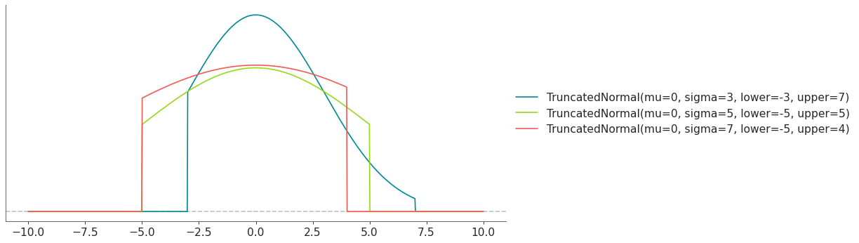
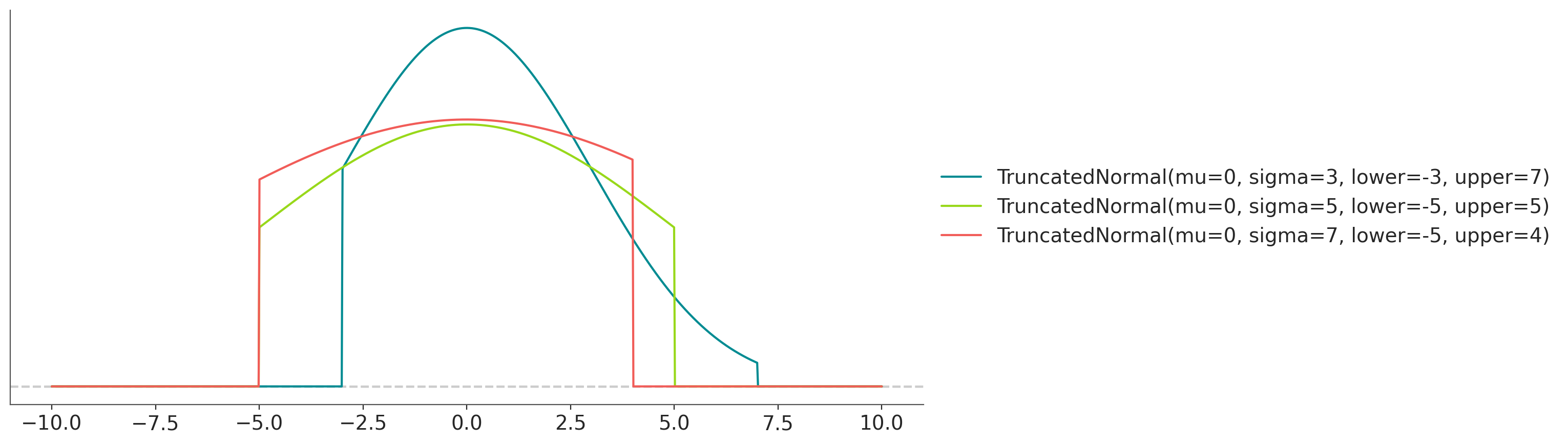
class preliz.distributions.uniform.Uniform(lower=None, upper=None)[source]#

Uniform distribution.

The pdf of this distribution is

\[f(x \mid lower, upper) = \frac{1}{upper-lower}\]

(Source code, png, hires.png, pdf)

Support	$x \in [lower, upper]$
Mean	$\dfrac{lower + upper}{2}$
Variance	$\dfrac{(upper - lower)^2}{12}$

Parameters:

lower (float) – Lower limit.
upper (float) – Upper limit (upper > lower).

cdf(x)[source]#

Cumulative distribution function.

Parameters:: x (array_like) – Values on which to evaluate the cdf

entropy()[source]#: Entropy.

eti(mass=None, fmt='.2f')#

Equal-tailed interval containing mass.

Parameters:

mass (float) – Probability mass in the interval. Defaults to None,
used. (which results in the value of rcParams["stats.ci_prob"] being)
fmt (str) – fmt used to represent results using f-string fmt for floats. Default to “.2f” i.e. 2 digits after the decimal point. Use “none” for no format.

hdi(mass=None, fmt='.2f')#

Highest density interval containing mass.

Parameters:

mass (float) – Probability mass in the interval. Defaults to None,
used. (which results in the value of rcParams["stats.ci_prob"] being)
fmt (str) – fmt used to represent results using f-string fmt for floats. Default to “.2f” i.e. 2 digits after the decimal point. Use “none” for no format.

isf(x)#

Inverse survival function (inverse of sf).

Parameters:: x (array_like) – Values on which to evaluate the inverse of the sf

kurtosis()[source]#: Excess kurtosis.

lmoment1()[source]#: L-moment1 (mean).

lmoment2()[source]#: L-moment2 (l-scale).

lmoment3()[source]#: L-moment3 (l-skewness). This the ratio of L-moment3 to L-moment2.

lmoment4()[source]#: L-moment4 (l-kurtosis). This the ratio of L-moment4 to L-moment2.

lmoments(types='1234')#

Compute L-moments of the distribution.

Parameters:: types (str) – The type of moments to compute. Default is ‘1234’ where ‘1’ = L-moment1 (mean), ‘2’ = L-moment2 (l-scale), ‘3’ = L-moment3 (l-skewness), and ‘4’ = L-moment4 (l-kurtosis). To compute the standard deviation use ‘d’ Valid combinations are any subset of ‘1234’.

logcdf(x)#

Log cumulative distribution function.

Parameters:: x (array_like) – Values on which to evaluate the logcdf

logpdf(x)[source]#

Log probability density/mass function.

Parameters:: x (array_like) – Values on which to evaluate the logpdf

logsf(x)#

Log survival function log(1 - cdf).

Parameters:: x (array_like) – Values on which to evaluate the logsf

mean()[source]#: Mean.

median()[source]#: Median.

mode()[source]#: Mode.

moments(types='mvsk')#

Compute moments of the distribution.

It can also return the standard deviation

Parameters:: types (str) – The type of moments to compute. Default is ‘mvsk’ where ‘m’ = mean, ‘v’ = variance, ‘s’ = skewness, and ‘k’ = kurtosis. To compute the standard deviation use ‘d’ Valid combinations are any subset of ‘mvdsk’.

pdf(x)[source]#

Probability density/mass function.

Parameters:: x (array_like) – Values on which to evaluate the pdf

plot_cdf(moments=None, pointinterval=False, interval=None, levels=None, support='restricted', legend='legend', figsize=None, ax=None, **kwargs)#

Plot the cumulative distribution function.

Parameters:

moments (str) – Compute moments. Use any combination of the strings m, d, v, s or k for the mean (μ), standard deviation (σ), variance (σ²), skew (γ) or kurtosis (κ) respectively. Other strings will be ignored. Defaults to None.
pointinterval (bool) – Whether to include a plot of the quantiles. Defaults to False. If True the default is to plot the median and two interquantiles ranges.
interval (str) – Type of interval. Available options are highest density interval “hdi” (default), equal tailed interval “eti” or intervals defined by arbitrary “quantiles”. Defaults to the value in rcParams[“stats.ci_kind”].
levels (list) – Mass of the intervals. For hdi or eti the number of elements should be 2 or 1. For quantiles the number of elements should be 5, 3, 1 or 0 (in this last case nothing will be plotted).
support (str:) – If full use the finite end-points to set the limits of the plot. For unbounded end-points or if restricted use the 0.001 and 0.999 quantiles to set the limits.
legend (str) – Whether to include a string with the distribution and its parameter as a "legend" a "title" or not include them None.
figsize (tuple) – Size of the figure
ax (matplotlib axes)
kwargs (keyword arguments) – Additional keyword arguments passed to matplotlib plot function. For example, color, alpha, linewidth, etc.

plot_interactive(kind='pdf', xy_lim='both', pointinterval=True, interval=None, levels=None, figsize=None)#

Interactive exploration of distributions parameters.

Parameters:

kind (str:) – Type of plot. Available options are pdf, cdf and ppf.
xy_lim (str or tuple) – Set the limits of the x-axis and/or y-axis. Defaults to “both”, the limits of both axis are fixed. Use “auto” for automatic rescaling of x-axis and y-axis. Or set them manually by passing a tuple of 4 elements, the first two for x-axis, the last two for y-axis. The tuple can have None.
pointinterval (bool) – Whether to include a plot of the quantiles. Defaults to False. If True the default is to plot the median and two interquantiles ranges.
interval (str) – Type of interval. Available options are highest density interval “hdi” (default), equal tailed interval “eti” or intervals defined by arbitrary “quantiles”. Defaults to the value in rcParams[“stats.ci_kind”].
levels (list) – Mass of the intervals. For hdi or eti the number of elements should be 2 or 1. For quantiles the number of elements should be 5, 3, 1 or 0 (in this last case nothing will be plotted).
figsize (tuple) – Size of the figure

plot_isf(moments=None, pointinterval=False, interval=None, levels=None, legend='legend', figsize=None, ax=None, **kwargs)#

Plot the inverse survival function.

Parameters:

moments (str) – Compute moments. Use any combination of the strings m, d, v, s or k for the mean (μ), standard deviation (σ), variance (σ²), skew (γ) or kurtosis (κ) respectively. Other strings will be ignored. Defaults to None.
pointinterval (bool) – Whether to include a plot of the quantiles. Defaults to False. If True the default is to plot the median and two interquantiles ranges.
interval (str) – Type of interval. Available options are highest density interval “hdi” (default), equal tailed interval “eti” or intervals defined by arbitrary “quantiles”. Defaults to the value in rcParams[“stats.ci_kind”].
levels (list) – Mass of the intervals. For hdi or eti the number of elements should be 2 or 1. For quantiles the number of elements should be 5, 3, 1 or 0 (in this last case nothing will be plotted).
legend (str) – Whether to include a string with the distribution and its parameter as a "legend" a "title" or not include them None.
figsize (tuple) – Size of the figure
ax (matplotlib axes)

plot_pdf(moments=None, pointinterval=False, interval=None, levels=None, support='restricted', baseline=True, legend='legend', figsize=None, ax=None, **kwargs)#

Plot the pdf (continuous) or pmf (discrete).

Parameters:

moments (str) – Compute moments. Use any combination of the strings m, d, v, s or k for the mean (μ), standard deviation (σ), variance (σ²), skew (γ) or kurtosis (κ) respectively. Other strings will be ignored. Defaults to None.
pointinterval (bool) – Whether to include a plot of the quantiles. Defaults to False. If True the default is to plot the median and two interquantiles ranges.
interval (str) – Type of interval. Available options are highest density interval “hdi” (default), equal tailed interval “eti” or intervals defined by arbitrary “quantiles”. Defaults to the value in rcParams[“stats.ci_kind”].
levels (list) – Mass of the intervals. For hdi or eti the number of elements should be 2 or 1. For quantiles the number of elements should be 5, 3, 1 or 0 (in this last case nothing will be plotted).
support (str:) – If full use the finite end-points to set the limits of the plot. For unbounded end-points or if restricted use the 0.001 and 0.999 quantiles to set the limits.
baseline (bool) – Whether to include a horizontal line at y=0.
legend (str) – Whether to include a string with the distribution and its parameter as a "legend" a "title" or not include them None.
figsize (tuple) – Size of the figure
ax (matplotlib axes)
kwargs (keyword arguments) – Additional keyword arguments passed to matplotlib plot function. For example, color, alpha, linewidth, etc.

plot_ppf(moments=None, pointinterval=False, interval=None, levels=None, legend='legend', figsize=None, ax=None, **kwargs)#

Plot the quantile function.

Parameters:

moments (str) – Compute moments. Use any combination of the strings m, d, v, s or k for the mean (μ), standard deviation (σ), variance (σ²), skew (γ) or kurtosis (κ) respectively. Other strings will be ignored. Defaults to None.
pointinterval (bool) – Whether to include a plot of the quantiles. Defaults to False. If True the default is to plot the median and two interquantiles ranges.
interval (str) – Type of interval. Available options are highest density interval “hdi” (default), equal tailed interval “eti” or intervals defined by arbitrary “quantiles”. Defaults to the value in rcParams[“stats.ci_kind”].
levels (list) – Mass of the intervals. For hdi or eti the number of elements should be 2 or 1. For quantiles the number of elements should be 5, 3, 1 or 0 (in this last case nothing will be plotted).
legend (str) – Whether to include a string with the distribution and its parameter as a "legend" a "title" or not include them None.
figsize (tuple) – Size of the figure
ax (matplotlib axes)

plot_sf(moments=None, pointinterval=False, interval=None, levels=None, support='restricted', legend='legend', figsize=None, ax=None, **kwargs)#

Plot the survival distribution function (1 - CDF).

Parameters:

moments (str) – Compute moments. Use any combination of the strings m, d, v, s or k for the mean (μ), standard deviation (σ), variance (σ²), skew (γ) or kurtosis (κ) respectively. Other strings will be ignored. Defaults to None.
pointinterval (bool) – Whether to include a plot of the quantiles. Defaults to False. If True the default is to plot the median and two interquantiles ranges.
interval (str) – Type of interval. Available options are highest density interval “hdi” (default), equal tailed interval “eti” or intervals defined by arbitrary “quantiles”. Defaults to the value in rcParams[“stats.ci_kind”].
levels (list) – Mass of the intervals. For hdi or eti the number of elements should be 2 or 1. For quantiles the number of elements should be 5, 3, 1 or 0 (in this last case nothing will be plotted).
support (str:) – If full use the finite end-points to set the limits of the plot. For unbounded end-points or if restricted use the 0.001 and 0.999 quantiles to set the limits.
legend (str) – Whether to include a string with the distribution and its parameter as a "legend" a "title" or not include them None.
figsize (tuple) – Size of the figure
ax (matplotlib axes)
kwargs (keyword arguments) – Additional keyword arguments passed to matplotlib plot function. For example, color, alpha, linewidth, etc.

ppf(q)[source]#

Percent point function (inverse of cdf).

Parameters:: x (array_like) – Values on which to evaluate the inverse of the cdf

rvs(size=None, random_state=None)[source]#

Random sample.

Parameters:

size (int or tuple of ints, optional) – Defining number of random variates. Defaults to 1.
random_state ({None, int, numpy.random.Generator, numpy.random.RandomState}) – Defaults to None

sf(x)#

Survival function (1 - cdf).

Parameters:: x (array_like) – Values on which to evaluate the sf

skewness()[source]#: Skewness.

std()[source]#: Standard deviation.

summary(mass=None, interval=None, fmt='.2f')#

Namedtuple with the mean, median, sd, and lower and upper bounds.

Parameters:

mass (float) – Probability mass for the equal-tailed interval. Defaults to None,
used. (which results in the value of rcParams["stats.ci_prob"] being)
interval (str or list-like) – Type of interval. Available options are highest density interval “hdi”, equal tailed interval “eti” or arbitrary interval defined by a list-like object with a pair of values. Defaults to the value in rcParams[“stats.ci_kind”].
fmt (str) – fmt used to represent results using f-string fmt for floats. Default to “.2f” i.e. 2 digits after the decimal point.

to_bambi(**kwargs)#

Convert the PreliZ distribution to a Bambi Prior.

kwargsPyMC distributions properties: kwargs are used to specify properties such as shape or dims

Return type:: Bambi Prior

to_pymc(name=None, **kwargs)#

Convert the PreliZ distribution to a PyMC distribution.

namestr: Name of PyMC distribution. Needed if inside Model context
kwargsPyMC distributions properties: kwargs are used to specify properties such as shape or dims

Return type:: PyMC distribution

var()[source]#: Variance.

xvals(support, n_points=None)#

Provide x values in the support of the distribution.

This is useful for example when plotting.

Parameters:

support (str) – Available options are “full” or “restricted”. If “full” the values will cover the entire support of the distribution if the boundary is finite, or the quantiles 0.0001 or 0.9999, if infinite. If “restricted” the values will cover the quantile 0.0001 to 0.9999.
n_points (int) – Number of values to return. Defaults to 1000 for continuous distributions and 200 for discrete ones. For discrete distributions the returned values may be fewer than n_points if the actual number of discrete values in the support of the distribution is smaller than n_points.

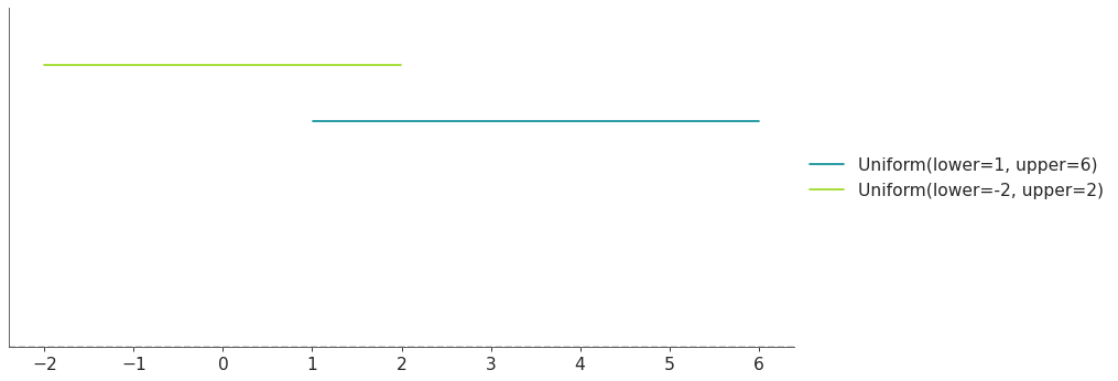
class preliz.distributions.vonmises.VonMises(mu=None, kappa=None)[source]#

Univariate VonMises distribution.

The pdf of this distribution is

\[f(x \mid \mu, \kappa) = \frac{e^{\kappa\cos(x-\mu)}}{2\pi I_0(\kappa)}\]

where $I_0$ is the modified Bessel function of order 0.

(Source code, png, hires.png, pdf)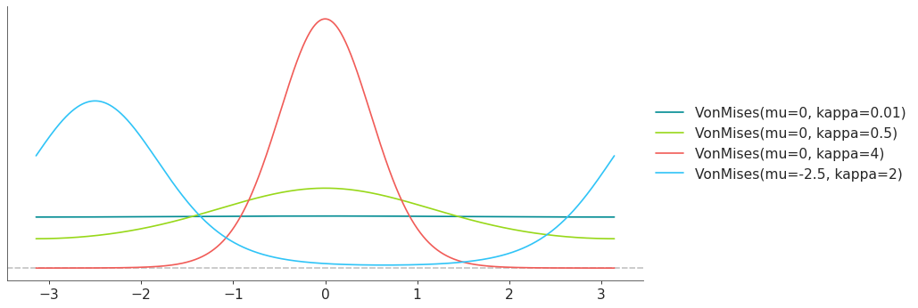

Support	$x \in [-\pi, \pi]$
Mean	$\mu$
Variance	$1-\frac{I_1(\kappa)}{I_0(\kappa)}$

Parameters:

mu (float) – Mean.
kappa (float) – Concentration ($\frac{1}{\kappa}$ is analogous to $\kappa^2$).

cdf(x)[source]#

Cumulative distribution function.

Parameters:: x (array_like) – Values on which to evaluate the cdf

entropy()[source]#: Entropy.

eti(mass=None, fmt='.2f')[source]#

Equal-tailed interval containing mass.

Parameters:

mass (float) – Probability mass in the interval. Defaults to None,
used. (which results in the value of rcParams["stats.ci_prob"] being)
fmt (str) – fmt used to represent results using f-string fmt for floats. Default to “.2f” i.e. 2 digits after the decimal point. Use “none” for no format.

hdi(mass=None, fmt='.2f')[source]#

Highest density interval containing mass.

Parameters:

mass (float) – Probability mass in the interval. Defaults to None,
used. (which results in the value of rcParams["stats.ci_prob"] being)
fmt (str) – fmt used to represent results using f-string fmt for floats. Default to “.2f” i.e. 2 digits after the decimal point. Use “none” for no format.

isf(x)#

Inverse survival function (inverse of sf).

Parameters:: x (array_like) – Values on which to evaluate the inverse of the sf

kurtosis()[source]#: Excess kurtosis.

lmoment1()[source]#: L-moment1 (mean).

lmoment2()[source]#: L-moment2 (l-scale).

lmoment3()[source]#: L-moment3 (l-skewness). This the ratio of L-moment3 to L-moment2.

lmoment4()[source]#: L-moment4 (l-kurtosis). This the ratio of L-moment4 to L-moment2.

lmoments(types='1234')#

Compute L-moments of the distribution.

Parameters:: types (str) – The type of moments to compute. Default is ‘1234’ where ‘1’ = L-moment1 (mean), ‘2’ = L-moment2 (l-scale), ‘3’ = L-moment3 (l-skewness), and ‘4’ = L-moment4 (l-kurtosis). To compute the standard deviation use ‘d’ Valid combinations are any subset of ‘1234’.

logcdf(x)#

Log cumulative distribution function.

Parameters:: x (array_like) – Values on which to evaluate the logcdf

logpdf(x)[source]#

Log probability density/mass function.

Parameters:: x (array_like) – Values on which to evaluate the logpdf

logsf(x)#

Log survival function log(1 - cdf).

Parameters:: x (array_like) – Values on which to evaluate the logsf

mean()[source]#: Mean.

median()[source]#: Median.

mode()[source]#: Mode.

moments(types='mvsk')#

Compute moments of the distribution.

It can also return the standard deviation

Parameters:: types (str) – The type of moments to compute. Default is ‘mvsk’ where ‘m’ = mean, ‘v’ = variance, ‘s’ = skewness, and ‘k’ = kurtosis. To compute the standard deviation use ‘d’ Valid combinations are any subset of ‘mvdsk’.

pdf(x)[source]#

Probability density/mass function.

Parameters:: x (array_like) – Values on which to evaluate the pdf

plot_cdf(moments=None, pointinterval=False, interval=None, levels=None, support='restricted', legend='legend', figsize=None, ax=None, **kwargs)#

Plot the cumulative distribution function.

Parameters:

moments (str) – Compute moments. Use any combination of the strings m, d, v, s or k for the mean (μ), standard deviation (σ), variance (σ²), skew (γ) or kurtosis (κ) respectively. Other strings will be ignored. Defaults to None.
pointinterval (bool) – Whether to include a plot of the quantiles. Defaults to False. If True the default is to plot the median and two interquantiles ranges.
interval (str) – Type of interval. Available options are highest density interval “hdi” (default), equal tailed interval “eti” or intervals defined by arbitrary “quantiles”. Defaults to the value in rcParams[“stats.ci_kind”].
levels (list) – Mass of the intervals. For hdi or eti the number of elements should be 2 or 1. For quantiles the number of elements should be 5, 3, 1 or 0 (in this last case nothing will be plotted).
support (str:) – If full use the finite end-points to set the limits of the plot. For unbounded end-points or if restricted use the 0.001 and 0.999 quantiles to set the limits.
legend (str) – Whether to include a string with the distribution and its parameter as a "legend" a "title" or not include them None.
figsize (tuple) – Size of the figure
ax (matplotlib axes)
kwargs (keyword arguments) – Additional keyword arguments passed to matplotlib plot function. For example, color, alpha, linewidth, etc.

plot_interactive(kind='pdf', xy_lim='both', pointinterval=True, interval=None, levels=None, figsize=None)#

Interactive exploration of distributions parameters.

Parameters:

kind (str:) – Type of plot. Available options are pdf, cdf and ppf.
xy_lim (str or tuple) – Set the limits of the x-axis and/or y-axis. Defaults to “both”, the limits of both axis are fixed. Use “auto” for automatic rescaling of x-axis and y-axis. Or set them manually by passing a tuple of 4 elements, the first two for x-axis, the last two for y-axis. The tuple can have None.
pointinterval (bool) – Whether to include a plot of the quantiles. Defaults to False. If True the default is to plot the median and two interquantiles ranges.
interval (str) – Type of interval. Available options are highest density interval “hdi” (default), equal tailed interval “eti” or intervals defined by arbitrary “quantiles”. Defaults to the value in rcParams[“stats.ci_kind”].
levels (list) – Mass of the intervals. For hdi or eti the number of elements should be 2 or 1. For quantiles the number of elements should be 5, 3, 1 or 0 (in this last case nothing will be plotted).
figsize (tuple) – Size of the figure

plot_isf(moments=None, pointinterval=False, interval=None, levels=None, legend='legend', figsize=None, ax=None, **kwargs)#

Plot the inverse survival function.

Parameters:

moments (str) – Compute moments. Use any combination of the strings m, d, v, s or k for the mean (μ), standard deviation (σ), variance (σ²), skew (γ) or kurtosis (κ) respectively. Other strings will be ignored. Defaults to None.
pointinterval (bool) – Whether to include a plot of the quantiles. Defaults to False. If True the default is to plot the median and two interquantiles ranges.
interval (str) – Type of interval. Available options are highest density interval “hdi” (default), equal tailed interval “eti” or intervals defined by arbitrary “quantiles”. Defaults to the value in rcParams[“stats.ci_kind”].
levels (list) – Mass of the intervals. For hdi or eti the number of elements should be 2 or 1. For quantiles the number of elements should be 5, 3, 1 or 0 (in this last case nothing will be plotted).
legend (str) – Whether to include a string with the distribution and its parameter as a "legend" a "title" or not include them None.
figsize (tuple) – Size of the figure
ax (matplotlib axes)

plot_pdf(moments=None, pointinterval=False, interval=None, levels=None, support='restricted', baseline=True, legend='legend', figsize=None, ax=None, **kwargs)#

Plot the pdf (continuous) or pmf (discrete).

Parameters:

moments (str) – Compute moments. Use any combination of the strings m, d, v, s or k for the mean (μ), standard deviation (σ), variance (σ²), skew (γ) or kurtosis (κ) respectively. Other strings will be ignored. Defaults to None.
pointinterval (bool) – Whether to include a plot of the quantiles. Defaults to False. If True the default is to plot the median and two interquantiles ranges.
interval (str) – Type of interval. Available options are highest density interval “hdi” (default), equal tailed interval “eti” or intervals defined by arbitrary “quantiles”. Defaults to the value in rcParams[“stats.ci_kind”].
levels (list) – Mass of the intervals. For hdi or eti the number of elements should be 2 or 1. For quantiles the number of elements should be 5, 3, 1 or 0 (in this last case nothing will be plotted).
support (str:) – If full use the finite end-points to set the limits of the plot. For unbounded end-points or if restricted use the 0.001 and 0.999 quantiles to set the limits.
baseline (bool) – Whether to include a horizontal line at y=0.
legend (str) – Whether to include a string with the distribution and its parameter as a "legend" a "title" or not include them None.
figsize (tuple) – Size of the figure
ax (matplotlib axes)
kwargs (keyword arguments) – Additional keyword arguments passed to matplotlib plot function. For example, color, alpha, linewidth, etc.

plot_ppf(moments=None, pointinterval=False, interval=None, levels=None, legend='legend', figsize=None, ax=None, **kwargs)#

Plot the quantile function.

Parameters:

moments (str) – Compute moments. Use any combination of the strings m, d, v, s or k for the mean (μ), standard deviation (σ), variance (σ²), skew (γ) or kurtosis (κ) respectively. Other strings will be ignored. Defaults to None.
pointinterval (bool) – Whether to include a plot of the quantiles. Defaults to False. If True the default is to plot the median and two interquantiles ranges.
interval (str) – Type of interval. Available options are highest density interval “hdi” (default), equal tailed interval “eti” or intervals defined by arbitrary “quantiles”. Defaults to the value in rcParams[“stats.ci_kind”].
levels (list) – Mass of the intervals. For hdi or eti the number of elements should be 2 or 1. For quantiles the number of elements should be 5, 3, 1 or 0 (in this last case nothing will be plotted).
legend (str) – Whether to include a string with the distribution and its parameter as a "legend" a "title" or not include them None.
figsize (tuple) – Size of the figure
ax (matplotlib axes)

plot_sf(moments=None, pointinterval=False, interval=None, levels=None, support='restricted', legend='legend', figsize=None, ax=None, **kwargs)#

Plot the survival distribution function (1 - CDF).

Parameters:

moments (str) – Compute moments. Use any combination of the strings m, d, v, s or k for the mean (μ), standard deviation (σ), variance (σ²), skew (γ) or kurtosis (κ) respectively. Other strings will be ignored. Defaults to None.
pointinterval (bool) – Whether to include a plot of the quantiles. Defaults to False. If True the default is to plot the median and two interquantiles ranges.
interval (str) – Type of interval. Available options are highest density interval “hdi” (default), equal tailed interval “eti” or intervals defined by arbitrary “quantiles”. Defaults to the value in rcParams[“stats.ci_kind”].
levels (list) – Mass of the intervals. For hdi or eti the number of elements should be 2 or 1. For quantiles the number of elements should be 5, 3, 1 or 0 (in this last case nothing will be plotted).
support (str:) – If full use the finite end-points to set the limits of the plot. For unbounded end-points or if restricted use the 0.001 and 0.999 quantiles to set the limits.
legend (str) – Whether to include a string with the distribution and its parameter as a "legend" a "title" or not include them None.
figsize (tuple) – Size of the figure
ax (matplotlib axes)
kwargs (keyword arguments) – Additional keyword arguments passed to matplotlib plot function. For example, color, alpha, linewidth, etc.

ppf(q)[source]#

Percent point function (inverse of cdf).

Parameters:: x (array_like) – Values on which to evaluate the inverse of the cdf

rvs(size=None, random_state=None)[source]#

Random sample.

Parameters:

size (int or tuple of ints, optional) – Defining number of random variates. Defaults to 1.
random_state ({None, int, numpy.random.Generator, numpy.random.RandomState}) – Defaults to None

sf(x)#

Survival function (1 - cdf).

Parameters:: x (array_like) – Values on which to evaluate the sf

skewness()[source]#: Skewness.

std()[source]#: Standard deviation.

summary(mass=None, interval=None, fmt='.2f')#

Namedtuple with the mean, median, sd, and lower and upper bounds.

Parameters:

mass (float) – Probability mass for the equal-tailed interval. Defaults to None,
used. (which results in the value of rcParams["stats.ci_prob"] being)
interval (str or list-like) – Type of interval. Available options are highest density interval “hdi”, equal tailed interval “eti” or arbitrary interval defined by a list-like object with a pair of values. Defaults to the value in rcParams[“stats.ci_kind”].
fmt (str) – fmt used to represent results using f-string fmt for floats. Default to “.2f” i.e. 2 digits after the decimal point.

to_bambi(**kwargs)#

Convert the PreliZ distribution to a Bambi Prior.

kwargsPyMC distributions properties: kwargs are used to specify properties such as shape or dims

Return type:: Bambi Prior

to_pymc(name=None, **kwargs)#

Convert the PreliZ distribution to a PyMC distribution.

namestr: Name of PyMC distribution. Needed if inside Model context
kwargsPyMC distributions properties: kwargs are used to specify properties such as shape or dims

Return type:: PyMC distribution

var()[source]#: Variance.

xvals(support, n_points=None)#

Provide x values in the support of the distribution.

This is useful for example when plotting.

Parameters:

support (str) – Available options are “full” or “restricted”. If “full” the values will cover the entire support of the distribution if the boundary is finite, or the quantiles 0.0001 or 0.9999, if infinite. If “restricted” the values will cover the quantile 0.0001 to 0.9999.
n_points (int) – Number of values to return. Defaults to 1000 for continuous distributions and 200 for discrete ones. For discrete distributions the returned values may be fewer than n_points if the actual number of discrete values in the support of the distribution is smaller than n_points.

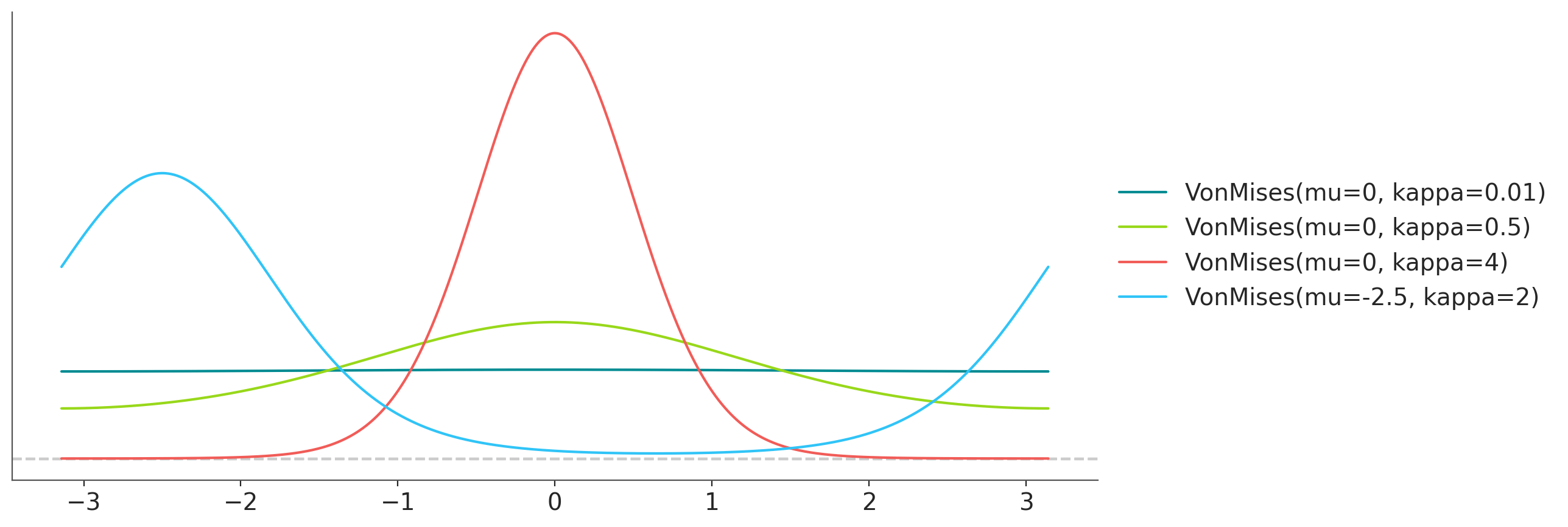
class preliz.distributions.wald.Wald(mu=None, lam=None, phi=None)[source]#

Wald distribution.

The pdf of this distribution is

\[f(x \mid \mu, \lambda) = \left(\frac{\lambda}{2\pi}\right)^{1/2} x^{-3/2} \exp\left\{ -\frac{\lambda}{2x}\left(\frac{x-\mu}{\mu}\right)^2 \right\}\]

(Source code, png, hires.png, pdf)

Support	$x \in (0, \infty)$
Mean	$\mu$
Variance	$\dfrac{\mu^3}{\lambda}$

Wald distribution has 3 alternative parametrizations. In terms of mu and lam, mu and phi or lam and phi.

The link between the 3 alternatives is given by

\[\phi = \dfrac{\lambda}{\mu}\]

Parameters:

mu (float) – Mean of the distribution (mu > 0).
lam (float) – Relative precision (lam > 0).
phi (float) – Shape parameter (phi > 0).

cdf(x)[source]#

Cumulative distribution function.

Parameters:: x (array_like) – Values on which to evaluate the cdf

entropy()[source]#: Entropy.

eti(mass=None, fmt='.2f')#

Equal-tailed interval containing mass.

Parameters:

mass (float) – Probability mass in the interval. Defaults to None,
used. (which results in the value of rcParams["stats.ci_prob"] being)
fmt (str) – fmt used to represent results using f-string fmt for floats. Default to “.2f” i.e. 2 digits after the decimal point. Use “none” for no format.

hdi(mass=None, fmt='.2f')#

Highest density interval containing mass.

Parameters:

mass (float) – Probability mass in the interval. Defaults to None,
used. (which results in the value of rcParams["stats.ci_prob"] being)
fmt (str) – fmt used to represent results using f-string fmt for floats. Default to “.2f” i.e. 2 digits after the decimal point. Use “none” for no format.

isf(x)#

Inverse survival function (inverse of sf).

Parameters:: x (array_like) – Values on which to evaluate the inverse of the sf

kurtosis()[source]#: Excess kurtosis.

lmoment1()[source]#: L-moment1 (mean).

lmoment2()[source]#: L-moment2 (l-scale).

lmoment3()[source]#: L-moment3 (l-skewness). This the ratio of L-moment3 to L-moment2.

lmoment4()[source]#: L-moment4 (l-kurtosis). This the ratio of L-moment4 to L-moment2.

lmoments(types='1234')#

Compute L-moments of the distribution.

Parameters:: types (str) – The type of moments to compute. Default is ‘1234’ where ‘1’ = L-moment1 (mean), ‘2’ = L-moment2 (l-scale), ‘3’ = L-moment3 (l-skewness), and ‘4’ = L-moment4 (l-kurtosis). To compute the standard deviation use ‘d’ Valid combinations are any subset of ‘1234’.

logcdf(x)#

Log cumulative distribution function.

Parameters:: x (array_like) – Values on which to evaluate the logcdf

logpdf(x)[source]#

Log probability density/mass function.

Parameters:: x (array_like) – Values on which to evaluate the logpdf

logsf(x)#

Log survival function log(1 - cdf).

Parameters:: x (array_like) – Values on which to evaluate the logsf

mean()[source]#: Mean.

median()[source]#: Median.

mode()[source]#: Mode.

moments(types='mvsk')#

Compute moments of the distribution.

It can also return the standard deviation

Parameters:: types (str) – The type of moments to compute. Default is ‘mvsk’ where ‘m’ = mean, ‘v’ = variance, ‘s’ = skewness, and ‘k’ = kurtosis. To compute the standard deviation use ‘d’ Valid combinations are any subset of ‘mvdsk’.

pdf(x)[source]#

Probability density/mass function.

Parameters:: x (array_like) – Values on which to evaluate the pdf

plot_cdf(moments=None, pointinterval=False, interval=None, levels=None, support='restricted', legend='legend', figsize=None, ax=None, **kwargs)#

Plot the cumulative distribution function.

Parameters:

moments (str) – Compute moments. Use any combination of the strings m, d, v, s or k for the mean (μ), standard deviation (σ), variance (σ²), skew (γ) or kurtosis (κ) respectively. Other strings will be ignored. Defaults to None.
pointinterval (bool) – Whether to include a plot of the quantiles. Defaults to False. If True the default is to plot the median and two interquantiles ranges.
interval (str) – Type of interval. Available options are highest density interval “hdi” (default), equal tailed interval “eti” or intervals defined by arbitrary “quantiles”. Defaults to the value in rcParams[“stats.ci_kind”].
levels (list) – Mass of the intervals. For hdi or eti the number of elements should be 2 or 1. For quantiles the number of elements should be 5, 3, 1 or 0 (in this last case nothing will be plotted).
support (str:) – If full use the finite end-points to set the limits of the plot. For unbounded end-points or if restricted use the 0.001 and 0.999 quantiles to set the limits.
legend (str) – Whether to include a string with the distribution and its parameter as a "legend" a "title" or not include them None.
figsize (tuple) – Size of the figure
ax (matplotlib axes)
kwargs (keyword arguments) – Additional keyword arguments passed to matplotlib plot function. For example, color, alpha, linewidth, etc.

plot_interactive(kind='pdf', xy_lim='both', pointinterval=True, interval=None, levels=None, figsize=None)#

Interactive exploration of distributions parameters.

Parameters:

kind (str:) – Type of plot. Available options are pdf, cdf and ppf.
xy_lim (str or tuple) – Set the limits of the x-axis and/or y-axis. Defaults to “both”, the limits of both axis are fixed. Use “auto” for automatic rescaling of x-axis and y-axis. Or set them manually by passing a tuple of 4 elements, the first two for x-axis, the last two for y-axis. The tuple can have None.
pointinterval (bool) – Whether to include a plot of the quantiles. Defaults to False. If True the default is to plot the median and two interquantiles ranges.
interval (str) – Type of interval. Available options are highest density interval “hdi” (default), equal tailed interval “eti” or intervals defined by arbitrary “quantiles”. Defaults to the value in rcParams[“stats.ci_kind”].
levels (list) – Mass of the intervals. For hdi or eti the number of elements should be 2 or 1. For quantiles the number of elements should be 5, 3, 1 or 0 (in this last case nothing will be plotted).
figsize (tuple) – Size of the figure

plot_isf(moments=None, pointinterval=False, interval=None, levels=None, legend='legend', figsize=None, ax=None, **kwargs)#

Plot the inverse survival function.

Parameters:

moments (str) – Compute moments. Use any combination of the strings m, d, v, s or k for the mean (μ), standard deviation (σ), variance (σ²), skew (γ) or kurtosis (κ) respectively. Other strings will be ignored. Defaults to None.
pointinterval (bool) – Whether to include a plot of the quantiles. Defaults to False. If True the default is to plot the median and two interquantiles ranges.
interval (str) – Type of interval. Available options are highest density interval “hdi” (default), equal tailed interval “eti” or intervals defined by arbitrary “quantiles”. Defaults to the value in rcParams[“stats.ci_kind”].
levels (list) – Mass of the intervals. For hdi or eti the number of elements should be 2 or 1. For quantiles the number of elements should be 5, 3, 1 or 0 (in this last case nothing will be plotted).
legend (str) – Whether to include a string with the distribution and its parameter as a "legend" a "title" or not include them None.
figsize (tuple) – Size of the figure
ax (matplotlib axes)

plot_pdf(moments=None, pointinterval=False, interval=None, levels=None, support='restricted', baseline=True, legend='legend', figsize=None, ax=None, **kwargs)#

Plot the pdf (continuous) or pmf (discrete).

Parameters:

moments (str) – Compute moments. Use any combination of the strings m, d, v, s or k for the mean (μ), standard deviation (σ), variance (σ²), skew (γ) or kurtosis (κ) respectively. Other strings will be ignored. Defaults to None.
pointinterval (bool) – Whether to include a plot of the quantiles. Defaults to False. If True the default is to plot the median and two interquantiles ranges.
interval (str) – Type of interval. Available options are highest density interval “hdi” (default), equal tailed interval “eti” or intervals defined by arbitrary “quantiles”. Defaults to the value in rcParams[“stats.ci_kind”].
levels (list) – Mass of the intervals. For hdi or eti the number of elements should be 2 or 1. For quantiles the number of elements should be 5, 3, 1 or 0 (in this last case nothing will be plotted).
support (str:) – If full use the finite end-points to set the limits of the plot. For unbounded end-points or if restricted use the 0.001 and 0.999 quantiles to set the limits.
baseline (bool) – Whether to include a horizontal line at y=0.
legend (str) – Whether to include a string with the distribution and its parameter as a "legend" a "title" or not include them None.
figsize (tuple) – Size of the figure
ax (matplotlib axes)
kwargs (keyword arguments) – Additional keyword arguments passed to matplotlib plot function. For example, color, alpha, linewidth, etc.

plot_ppf(moments=None, pointinterval=False, interval=None, levels=None, legend='legend', figsize=None, ax=None, **kwargs)#

Plot the quantile function.

Parameters:

moments (str) – Compute moments. Use any combination of the strings m, d, v, s or k for the mean (μ), standard deviation (σ), variance (σ²), skew (γ) or kurtosis (κ) respectively. Other strings will be ignored. Defaults to None.
pointinterval (bool) – Whether to include a plot of the quantiles. Defaults to False. If True the default is to plot the median and two interquantiles ranges.
interval (str) – Type of interval. Available options are highest density interval “hdi” (default), equal tailed interval “eti” or intervals defined by arbitrary “quantiles”. Defaults to the value in rcParams[“stats.ci_kind”].
levels (list) – Mass of the intervals. For hdi or eti the number of elements should be 2 or 1. For quantiles the number of elements should be 5, 3, 1 or 0 (in this last case nothing will be plotted).
legend (str) – Whether to include a string with the distribution and its parameter as a "legend" a "title" or not include them None.
figsize (tuple) – Size of the figure
ax (matplotlib axes)

plot_sf(moments=None, pointinterval=False, interval=None, levels=None, support='restricted', legend='legend', figsize=None, ax=None, **kwargs)#

Plot the survival distribution function (1 - CDF).

Parameters:

moments (str) – Compute moments. Use any combination of the strings m, d, v, s or k for the mean (μ), standard deviation (σ), variance (σ²), skew (γ) or kurtosis (κ) respectively. Other strings will be ignored. Defaults to None.
pointinterval (bool) – Whether to include a plot of the quantiles. Defaults to False. If True the default is to plot the median and two interquantiles ranges.
interval (str) – Type of interval. Available options are highest density interval “hdi” (default), equal tailed interval “eti” or intervals defined by arbitrary “quantiles”. Defaults to the value in rcParams[“stats.ci_kind”].
levels (list) – Mass of the intervals. For hdi or eti the number of elements should be 2 or 1. For quantiles the number of elements should be 5, 3, 1 or 0 (in this last case nothing will be plotted).
support (str:) – If full use the finite end-points to set the limits of the plot. For unbounded end-points or if restricted use the 0.001 and 0.999 quantiles to set the limits.
legend (str) – Whether to include a string with the distribution and its parameter as a "legend" a "title" or not include them None.
figsize (tuple) – Size of the figure
ax (matplotlib axes)
kwargs (keyword arguments) – Additional keyword arguments passed to matplotlib plot function. For example, color, alpha, linewidth, etc.

ppf(q)[source]#

Percent point function (inverse of cdf).

Parameters:: x (array_like) – Values on which to evaluate the inverse of the cdf

rvs(size=None, random_state=None)[source]#

Random sample.

Parameters:

size (int or tuple of ints, optional) – Defining number of random variates. Defaults to 1.
random_state ({None, int, numpy.random.Generator, numpy.random.RandomState}) – Defaults to None

sf(x)#

Survival function (1 - cdf).

Parameters:: x (array_like) – Values on which to evaluate the sf

skewness()[source]#: Skewness.

std()[source]#: Standard deviation.

summary(mass=None, interval=None, fmt='.2f')#

Namedtuple with the mean, median, sd, and lower and upper bounds.

Parameters:

mass (float) – Probability mass for the equal-tailed interval. Defaults to None,
used. (which results in the value of rcParams["stats.ci_prob"] being)
interval (str or list-like) – Type of interval. Available options are highest density interval “hdi”, equal tailed interval “eti” or arbitrary interval defined by a list-like object with a pair of values. Defaults to the value in rcParams[“stats.ci_kind”].
fmt (str) – fmt used to represent results using f-string fmt for floats. Default to “.2f” i.e. 2 digits after the decimal point.

to_bambi(**kwargs)#

Convert the PreliZ distribution to a Bambi Prior.

kwargsPyMC distributions properties: kwargs are used to specify properties such as shape or dims

Return type:: Bambi Prior

to_pymc(name=None, **kwargs)#

Convert the PreliZ distribution to a PyMC distribution.

namestr: Name of PyMC distribution. Needed if inside Model context
kwargsPyMC distributions properties: kwargs are used to specify properties such as shape or dims

Return type:: PyMC distribution

var()[source]#: Variance.

xvals(support, n_points=None)#

Provide x values in the support of the distribution.

This is useful for example when plotting.

Parameters:

support (str) – Available options are “full” or “restricted”. If “full” the values will cover the entire support of the distribution if the boundary is finite, or the quantiles 0.0001 or 0.9999, if infinite. If “restricted” the values will cover the quantile 0.0001 to 0.9999.
n_points (int) – Number of values to return. Defaults to 1000 for continuous distributions and 200 for discrete ones. For discrete distributions the returned values may be fewer than n_points if the actual number of discrete values in the support of the distribution is smaller than n_points.

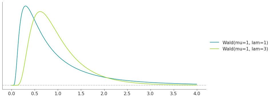
class preliz.distributions.weibull.Weibull(alpha=None, beta=None)[source]#

Weibull distribution.

The pdf of this distribution is

\[f(x \mid \alpha, \beta) = \frac{\alpha x^{\alpha - 1} \exp(-(\frac{x}{\beta})^{\alpha})}{\beta^\alpha}\]

(Source code, png, hires.png, pdf)

Support	$x \in [0, \infty)$
Mean	$\beta \Gamma(1 + \frac{1}{\alpha})$
Variance	$\beta^2 \Gamma(1 + \frac{2}{\alpha} - \mu^2/\beta^2)$

Parameters:

alpha (float) – Shape parameter (alpha > 0).
beta (float) – Scale parameter (beta > 0).

cdf(x)[source]#

Cumulative distribution function.

Parameters:: x (array_like) – Values on which to evaluate the cdf

entropy()[source]#: Entropy.

eti(mass=None, fmt='.2f')#

Equal-tailed interval containing mass.

Parameters:

mass (float) – Probability mass in the interval. Defaults to None,
used. (which results in the value of rcParams["stats.ci_prob"] being)
fmt (str) – fmt used to represent results using f-string fmt for floats. Default to “.2f” i.e. 2 digits after the decimal point. Use “none” for no format.

hdi(mass=None, fmt='.2f')#

Highest density interval containing mass.

Parameters:

mass (float) – Probability mass in the interval. Defaults to None,
used. (which results in the value of rcParams["stats.ci_prob"] being)
fmt (str) – fmt used to represent results using f-string fmt for floats. Default to “.2f” i.e. 2 digits after the decimal point. Use “none” for no format.

isf(x)#

Inverse survival function (inverse of sf).

Parameters:: x (array_like) – Values on which to evaluate the inverse of the sf

kurtosis()[source]#: Excess kurtosis.

lmoment1()[source]#: L-moment1 (mean).

lmoment2()[source]#: L-moment2 (l-scale).

lmoment3()[source]#: L-moment3 (l-skewness). This the ratio of L-moment3 to L-moment2.

lmoment4()[source]#: L-moment4 (l-kurtosis). This the ratio of L-moment4 to L-moment2.

lmoments(types='1234')#

Compute L-moments of the distribution.

Parameters:: types (str) – The type of moments to compute. Default is ‘1234’ where ‘1’ = L-moment1 (mean), ‘2’ = L-moment2 (l-scale), ‘3’ = L-moment3 (l-skewness), and ‘4’ = L-moment4 (l-kurtosis). To compute the standard deviation use ‘d’ Valid combinations are any subset of ‘1234’.

logcdf(x)#

Log cumulative distribution function.

Parameters:: x (array_like) – Values on which to evaluate the logcdf

logpdf(x)[source]#

Log probability density/mass function.

Parameters:: x (array_like) – Values on which to evaluate the logpdf

logsf(x)#

Log survival function log(1 - cdf).

Parameters:: x (array_like) – Values on which to evaluate the logsf

mean()[source]#: Mean.

median()[source]#: Median.

mode()[source]#: Mode.

moments(types='mvsk')#

Compute moments of the distribution.

It can also return the standard deviation

Parameters:: types (str) – The type of moments to compute. Default is ‘mvsk’ where ‘m’ = mean, ‘v’ = variance, ‘s’ = skewness, and ‘k’ = kurtosis. To compute the standard deviation use ‘d’ Valid combinations are any subset of ‘mvdsk’.

pdf(x)[source]#

Probability density/mass function.

Parameters:: x (array_like) – Values on which to evaluate the pdf

plot_cdf(moments=None, pointinterval=False, interval=None, levels=None, support='restricted', legend='legend', figsize=None, ax=None, **kwargs)#

Plot the cumulative distribution function.

Parameters:

moments (str) – Compute moments. Use any combination of the strings m, d, v, s or k for the mean (μ), standard deviation (σ), variance (σ²), skew (γ) or kurtosis (κ) respectively. Other strings will be ignored. Defaults to None.
pointinterval (bool) – Whether to include a plot of the quantiles. Defaults to False. If True the default is to plot the median and two interquantiles ranges.
interval (str) – Type of interval. Available options are highest density interval “hdi” (default), equal tailed interval “eti” or intervals defined by arbitrary “quantiles”. Defaults to the value in rcParams[“stats.ci_kind”].
levels (list) – Mass of the intervals. For hdi or eti the number of elements should be 2 or 1. For quantiles the number of elements should be 5, 3, 1 or 0 (in this last case nothing will be plotted).
support (str:) – If full use the finite end-points to set the limits of the plot. For unbounded end-points or if restricted use the 0.001 and 0.999 quantiles to set the limits.
legend (str) – Whether to include a string with the distribution and its parameter as a "legend" a "title" or not include them None.
figsize (tuple) – Size of the figure
ax (matplotlib axes)
kwargs (keyword arguments) – Additional keyword arguments passed to matplotlib plot function. For example, color, alpha, linewidth, etc.

plot_interactive(kind='pdf', xy_lim='both', pointinterval=True, interval=None, levels=None, figsize=None)#

Interactive exploration of distributions parameters.

Parameters:

kind (str:) – Type of plot. Available options are pdf, cdf and ppf.
xy_lim (str or tuple) – Set the limits of the x-axis and/or y-axis. Defaults to “both”, the limits of both axis are fixed. Use “auto” for automatic rescaling of x-axis and y-axis. Or set them manually by passing a tuple of 4 elements, the first two for x-axis, the last two for y-axis. The tuple can have None.
pointinterval (bool) – Whether to include a plot of the quantiles. Defaults to False. If True the default is to plot the median and two interquantiles ranges.
interval (str) – Type of interval. Available options are highest density interval “hdi” (default), equal tailed interval “eti” or intervals defined by arbitrary “quantiles”. Defaults to the value in rcParams[“stats.ci_kind”].
levels (list) – Mass of the intervals. For hdi or eti the number of elements should be 2 or 1. For quantiles the number of elements should be 5, 3, 1 or 0 (in this last case nothing will be plotted).
figsize (tuple) – Size of the figure

plot_isf(moments=None, pointinterval=False, interval=None, levels=None, legend='legend', figsize=None, ax=None, **kwargs)#

Plot the inverse survival function.

Parameters:

moments (str) – Compute moments. Use any combination of the strings m, d, v, s or k for the mean (μ), standard deviation (σ), variance (σ²), skew (γ) or kurtosis (κ) respectively. Other strings will be ignored. Defaults to None.
pointinterval (bool) – Whether to include a plot of the quantiles. Defaults to False. If True the default is to plot the median and two interquantiles ranges.
interval (str) – Type of interval. Available options are highest density interval “hdi” (default), equal tailed interval “eti” or intervals defined by arbitrary “quantiles”. Defaults to the value in rcParams[“stats.ci_kind”].
levels (list) – Mass of the intervals. For hdi or eti the number of elements should be 2 or 1. For quantiles the number of elements should be 5, 3, 1 or 0 (in this last case nothing will be plotted).
legend (str) – Whether to include a string with the distribution and its parameter as a "legend" a "title" or not include them None.
figsize (tuple) – Size of the figure
ax (matplotlib axes)

plot_pdf(moments=None, pointinterval=False, interval=None, levels=None, support='restricted', baseline=True, legend='legend', figsize=None, ax=None, **kwargs)#

Plot the pdf (continuous) or pmf (discrete).

Parameters:

moments (str) – Compute moments. Use any combination of the strings m, d, v, s or k for the mean (μ), standard deviation (σ), variance (σ²), skew (γ) or kurtosis (κ) respectively. Other strings will be ignored. Defaults to None.
pointinterval (bool) – Whether to include a plot of the quantiles. Defaults to False. If True the default is to plot the median and two interquantiles ranges.
interval (str) – Type of interval. Available options are highest density interval “hdi” (default), equal tailed interval “eti” or intervals defined by arbitrary “quantiles”. Defaults to the value in rcParams[“stats.ci_kind”].
levels (list) – Mass of the intervals. For hdi or eti the number of elements should be 2 or 1. For quantiles the number of elements should be 5, 3, 1 or 0 (in this last case nothing will be plotted).
support (str:) – If full use the finite end-points to set the limits of the plot. For unbounded end-points or if restricted use the 0.001 and 0.999 quantiles to set the limits.
baseline (bool) – Whether to include a horizontal line at y=0.
legend (str) – Whether to include a string with the distribution and its parameter as a "legend" a "title" or not include them None.
figsize (tuple) – Size of the figure
ax (matplotlib axes)
kwargs (keyword arguments) – Additional keyword arguments passed to matplotlib plot function. For example, color, alpha, linewidth, etc.

plot_ppf(moments=None, pointinterval=False, interval=None, levels=None, legend='legend', figsize=None, ax=None, **kwargs)#

Plot the quantile function.

Parameters:

moments (str) – Compute moments. Use any combination of the strings m, d, v, s or k for the mean (μ), standard deviation (σ), variance (σ²), skew (γ) or kurtosis (κ) respectively. Other strings will be ignored. Defaults to None.
pointinterval (bool) – Whether to include a plot of the quantiles. Defaults to False. If True the default is to plot the median and two interquantiles ranges.
interval (str) – Type of interval. Available options are highest density interval “hdi” (default), equal tailed interval “eti” or intervals defined by arbitrary “quantiles”. Defaults to the value in rcParams[“stats.ci_kind”].
levels (list) – Mass of the intervals. For hdi or eti the number of elements should be 2 or 1. For quantiles the number of elements should be 5, 3, 1 or 0 (in this last case nothing will be plotted).
legend (str) – Whether to include a string with the distribution and its parameter as a "legend" a "title" or not include them None.
figsize (tuple) – Size of the figure
ax (matplotlib axes)

plot_sf(moments=None, pointinterval=False, interval=None, levels=None, support='restricted', legend='legend', figsize=None, ax=None, **kwargs)#

Plot the survival distribution function (1 - CDF).

Parameters:

moments (str) – Compute moments. Use any combination of the strings m, d, v, s or k for the mean (μ), standard deviation (σ), variance (σ²), skew (γ) or kurtosis (κ) respectively. Other strings will be ignored. Defaults to None.
pointinterval (bool) – Whether to include a plot of the quantiles. Defaults to False. If True the default is to plot the median and two interquantiles ranges.
interval (str) – Type of interval. Available options are highest density interval “hdi” (default), equal tailed interval “eti” or intervals defined by arbitrary “quantiles”. Defaults to the value in rcParams[“stats.ci_kind”].
levels (list) – Mass of the intervals. For hdi or eti the number of elements should be 2 or 1. For quantiles the number of elements should be 5, 3, 1 or 0 (in this last case nothing will be plotted).
support (str:) – If full use the finite end-points to set the limits of the plot. For unbounded end-points or if restricted use the 0.001 and 0.999 quantiles to set the limits.
legend (str) – Whether to include a string with the distribution and its parameter as a "legend" a "title" or not include them None.
figsize (tuple) – Size of the figure
ax (matplotlib axes)
kwargs (keyword arguments) – Additional keyword arguments passed to matplotlib plot function. For example, color, alpha, linewidth, etc.

ppf(q)[source]#

Percent point function (inverse of cdf).

Parameters:: x (array_like) – Values on which to evaluate the inverse of the cdf

rvs(size=None, random_state=None)[source]#

Random sample.

Parameters:

size (int or tuple of ints, optional) – Defining number of random variates. Defaults to 1.
random_state ({None, int, numpy.random.Generator, numpy.random.RandomState}) – Defaults to None

sf(x)#

Survival function (1 - cdf).

Parameters:: x (array_like) – Values on which to evaluate the sf

skewness()[source]#: Skewness.

std()[source]#: Standard deviation.

summary(mass=None, interval=None, fmt='.2f')#

Namedtuple with the mean, median, sd, and lower and upper bounds.

Parameters:

mass (float) – Probability mass for the equal-tailed interval. Defaults to None,
used. (which results in the value of rcParams["stats.ci_prob"] being)
interval (str or list-like) – Type of interval. Available options are highest density interval “hdi”, equal tailed interval “eti” or arbitrary interval defined by a list-like object with a pair of values. Defaults to the value in rcParams[“stats.ci_kind”].
fmt (str) – fmt used to represent results using f-string fmt for floats. Default to “.2f” i.e. 2 digits after the decimal point.

to_bambi(**kwargs)#

Convert the PreliZ distribution to a Bambi Prior.

kwargsPyMC distributions properties: kwargs are used to specify properties such as shape or dims

Return type:: Bambi Prior

to_pymc(name=None, **kwargs)#

Convert the PreliZ distribution to a PyMC distribution.

namestr: Name of PyMC distribution. Needed if inside Model context
kwargsPyMC distributions properties: kwargs are used to specify properties such as shape or dims

Return type:: PyMC distribution

var()[source]#: Variance.

xvals(support, n_points=None)#

Provide x values in the support of the distribution.

This is useful for example when plotting.

Parameters:

support (str) – Available options are “full” or “restricted”. If “full” the values will cover the entire support of the distribution if the boundary is finite, or the quantiles 0.0001 or 0.9999, if infinite. If “restricted” the values will cover the quantile 0.0001 to 0.9999.
n_points (int) – Number of values to return. Defaults to 1000 for continuous distributions and 200 for discrete ones. For discrete distributions the returned values may be fewer than n_points if the actual number of discrete values in the support of the distribution is smaller than n_points.

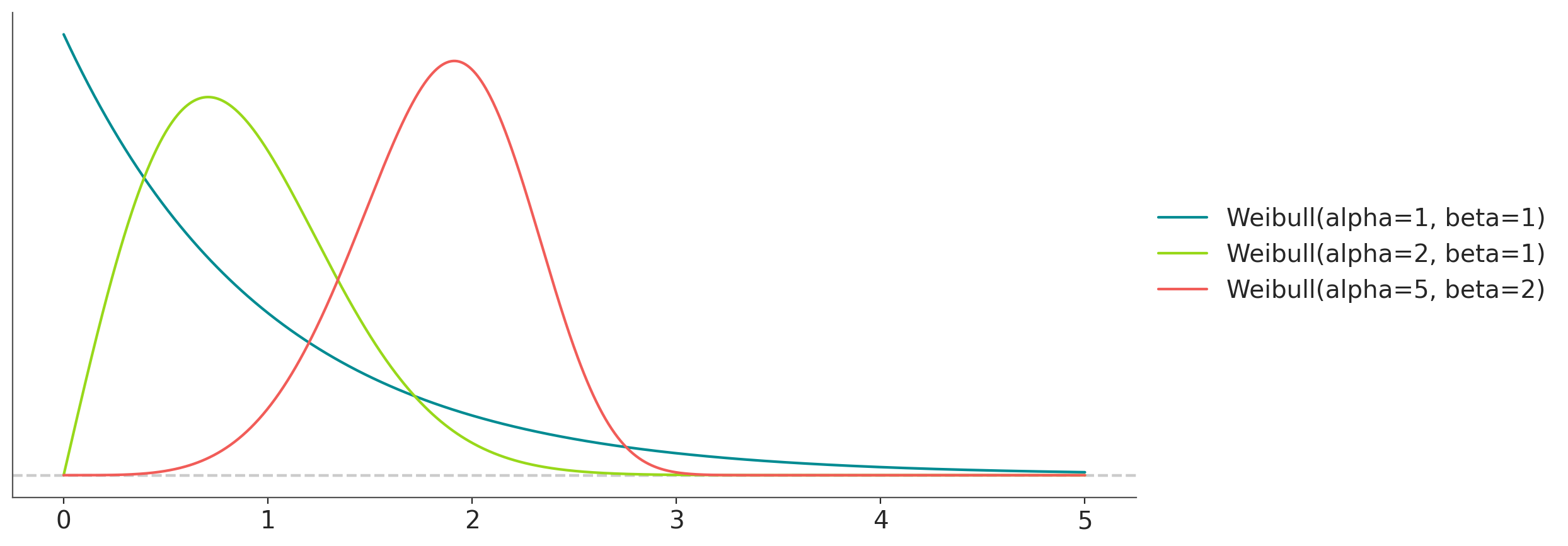
`preliz.distributions.discrete`#

class preliz.distributions.bernoulli.Bernoulli(p=None, logit_p=None)[source]#

Bernoulli distribution.

The Bernoulli distribution describes the probability of successes (x=1) and failures (x=0). The pmf of this distribution is

\[f(x \mid p) = p^{x} (1-p)^{1-x}\]

(Source code, png, hires.png, pdf)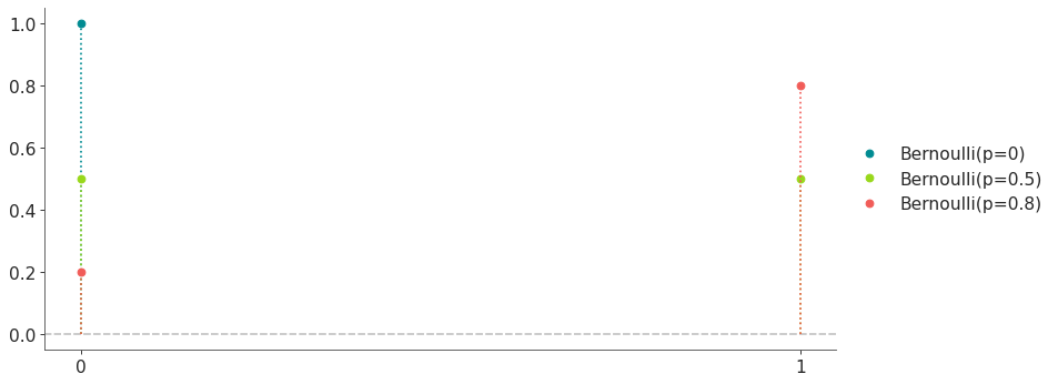

Support	$x \in \{0, 1\}$
Mean	$p$
Variance	$p (1 - p)$

The Bernoulli distribution has 2 alternative parametrizations. In terms of p or logit_p.

The link between the 2 alternatives is given by

\[logit(p) = ln(\frac{p}{1-p})\]

Parameters:

p (float) – Probability of success (0 < p < 1).
logit_p (float) – Alternative log odds for the probability of success.

cdf(x)[source]#

Cumulative distribution function.

Parameters:: x (array_like) – Values on which to evaluate the cdf

entropy()[source]#: Entropy.

eti(mass=None, fmt='.2f')#

Equal-tailed interval containing mass.

Parameters:

mass (float) – Probability mass in the interval. Defaults to None,
used. (which results in the value of rcParams["stats.ci_prob"] being)
fmt (str) – fmt used to represent results using f-string fmt for floats. Default to “.2f” i.e. 2 digits after the decimal point. Use “none” for no format.

hdi(mass=None, fmt='.2f')#

Highest density interval containing mass.

Parameters:

mass (float) – Probability mass in the interval. Defaults to None,
used. (which results in the value of rcParams["stats.ci_prob"] being)
fmt (str) – fmt used to represent results using f-string fmt for floats. Default to “.2f” i.e. 2 digits after the decimal point. Use “none” for no format.

isf(x)#

Inverse survival function (inverse of sf).

Parameters:: x (array_like) – Values on which to evaluate the inverse of the sf

kurtosis()[source]#: Excess kurtosis.

lmoment1()[source]#: L-moment1 (mean).

lmoment2()[source]#: L-moment2 (l-scale).

lmoment3()[source]#: L-moment3 (l-skewness). This the ratio of L-moment3 to L-moment2.

lmoment4()[source]#: L-moment4 (l-kurtosis). This the ratio of L-moment4 to L-moment2.

lmoments(types='1234')#

Compute L-moments of the distribution.

Parameters:: types (str) – The type of moments to compute. Default is ‘1234’ where ‘1’ = L-moment1 (mean), ‘2’ = L-moment2 (l-scale), ‘3’ = L-moment3 (l-skewness), and ‘4’ = L-moment4 (l-kurtosis). To compute the standard deviation use ‘d’ Valid combinations are any subset of ‘1234’.

logcdf(x)#

Log cumulative distribution function.

Parameters:: x (array_like) – Values on which to evaluate the logcdf

logpdf(x)[source]#

Log probability density/mass function.

Parameters:: x (array_like) – Values on which to evaluate the logpdf

logsf(x)#

Log survival function log(1 - cdf).

Parameters:: x (array_like) – Values on which to evaluate the logsf

mean()[source]#: Mean.

median()[source]#: Median.

mode()[source]#: Mode.

moments(types='mvsk')#

Compute moments of the distribution.

It can also return the standard deviation

Parameters:: types (str) – The type of moments to compute. Default is ‘mvsk’ where ‘m’ = mean, ‘v’ = variance, ‘s’ = skewness, and ‘k’ = kurtosis. To compute the standard deviation use ‘d’ Valid combinations are any subset of ‘mvdsk’.

pdf(x)[source]#

Probability density/mass function.

Parameters:: x (array_like) – Values on which to evaluate the pdf

plot_cdf(moments=None, pointinterval=False, interval=None, levels=None, support='restricted', legend='legend', figsize=None, ax=None, **kwargs)#

Plot the cumulative distribution function.

Parameters:

moments (str) – Compute moments. Use any combination of the strings m, d, v, s or k for the mean (μ), standard deviation (σ), variance (σ²), skew (γ) or kurtosis (κ) respectively. Other strings will be ignored. Defaults to None.
pointinterval (bool) – Whether to include a plot of the quantiles. Defaults to False. If True the default is to plot the median and two interquantiles ranges.
interval (str) – Type of interval. Available options are highest density interval “hdi” (default), equal tailed interval “eti” or intervals defined by arbitrary “quantiles”. Defaults to the value in rcParams[“stats.ci_kind”].
levels (list) – Mass of the intervals. For hdi or eti the number of elements should be 2 or 1. For quantiles the number of elements should be 5, 3, 1 or 0 (in this last case nothing will be plotted).
support (str:) – If full use the finite end-points to set the limits of the plot. For unbounded end-points or if restricted use the 0.001 and 0.999 quantiles to set the limits.
legend (str) – Whether to include a string with the distribution and its parameter as a "legend" a "title" or not include them None.
figsize (tuple) – Size of the figure
ax (matplotlib axes)
kwargs (keyword arguments) – Additional keyword arguments passed to matplotlib plot function. For example, color, alpha, linewidth, etc.

plot_interactive(kind='pdf', xy_lim='both', pointinterval=True, interval=None, levels=None, figsize=None)#

Interactive exploration of distributions parameters.

Parameters:

kind (str:) – Type of plot. Available options are pdf, cdf and ppf.
xy_lim (str or tuple) – Set the limits of the x-axis and/or y-axis. Defaults to “both”, the limits of both axis are fixed. Use “auto” for automatic rescaling of x-axis and y-axis. Or set them manually by passing a tuple of 4 elements, the first two for x-axis, the last two for y-axis. The tuple can have None.
pointinterval (bool) – Whether to include a plot of the quantiles. Defaults to False. If True the default is to plot the median and two interquantiles ranges.
interval (str) – Type of interval. Available options are highest density interval “hdi” (default), equal tailed interval “eti” or intervals defined by arbitrary “quantiles”. Defaults to the value in rcParams[“stats.ci_kind”].
levels (list) – Mass of the intervals. For hdi or eti the number of elements should be 2 or 1. For quantiles the number of elements should be 5, 3, 1 or 0 (in this last case nothing will be plotted).
figsize (tuple) – Size of the figure

plot_isf(moments=None, pointinterval=False, interval=None, levels=None, legend='legend', figsize=None, ax=None, **kwargs)#

Plot the inverse survival function.

Parameters:

moments (str) – Compute moments. Use any combination of the strings m, d, v, s or k for the mean (μ), standard deviation (σ), variance (σ²), skew (γ) or kurtosis (κ) respectively. Other strings will be ignored. Defaults to None.
pointinterval (bool) – Whether to include a plot of the quantiles. Defaults to False. If True the default is to plot the median and two interquantiles ranges.
interval (str) – Type of interval. Available options are highest density interval “hdi” (default), equal tailed interval “eti” or intervals defined by arbitrary “quantiles”. Defaults to the value in rcParams[“stats.ci_kind”].
levels (list) – Mass of the intervals. For hdi or eti the number of elements should be 2 or 1. For quantiles the number of elements should be 5, 3, 1 or 0 (in this last case nothing will be plotted).
legend (str) – Whether to include a string with the distribution and its parameter as a "legend" a "title" or not include them None.
figsize (tuple) – Size of the figure
ax (matplotlib axes)

plot_pdf(moments=None, pointinterval=False, interval=None, levels=None, support='restricted', baseline=True, legend='legend', figsize=None, ax=None, **kwargs)#

Plot the pdf (continuous) or pmf (discrete).

Parameters:

moments (str) – Compute moments. Use any combination of the strings m, d, v, s or k for the mean (μ), standard deviation (σ), variance (σ²), skew (γ) or kurtosis (κ) respectively. Other strings will be ignored. Defaults to None.
pointinterval (bool) – Whether to include a plot of the quantiles. Defaults to False. If True the default is to plot the median and two interquantiles ranges.
interval (str) – Type of interval. Available options are highest density interval “hdi” (default), equal tailed interval “eti” or intervals defined by arbitrary “quantiles”. Defaults to the value in rcParams[“stats.ci_kind”].
levels (list) – Mass of the intervals. For hdi or eti the number of elements should be 2 or 1. For quantiles the number of elements should be 5, 3, 1 or 0 (in this last case nothing will be plotted).
support (str:) – If full use the finite end-points to set the limits of the plot. For unbounded end-points or if restricted use the 0.001 and 0.999 quantiles to set the limits.
baseline (bool) – Whether to include a horizontal line at y=0.
legend (str) – Whether to include a string with the distribution and its parameter as a "legend" a "title" or not include them None.
figsize (tuple) – Size of the figure
ax (matplotlib axes)
kwargs (keyword arguments) – Additional keyword arguments passed to matplotlib plot function. For example, color, alpha, linewidth, etc.

plot_ppf(moments=None, pointinterval=False, interval=None, levels=None, legend='legend', figsize=None, ax=None, **kwargs)#

Plot the quantile function.

Parameters:

moments (str) – Compute moments. Use any combination of the strings m, d, v, s or k for the mean (μ), standard deviation (σ), variance (σ²), skew (γ) or kurtosis (κ) respectively. Other strings will be ignored. Defaults to None.
pointinterval (bool) – Whether to include a plot of the quantiles. Defaults to False. If True the default is to plot the median and two interquantiles ranges.
interval (str) – Type of interval. Available options are highest density interval “hdi” (default), equal tailed interval “eti” or intervals defined by arbitrary “quantiles”. Defaults to the value in rcParams[“stats.ci_kind”].
levels (list) – Mass of the intervals. For hdi or eti the number of elements should be 2 or 1. For quantiles the number of elements should be 5, 3, 1 or 0 (in this last case nothing will be plotted).
legend (str) – Whether to include a string with the distribution and its parameter as a "legend" a "title" or not include them None.
figsize (tuple) – Size of the figure
ax (matplotlib axes)

plot_sf(moments=None, pointinterval=False, interval=None, levels=None, support='restricted', legend='legend', figsize=None, ax=None, **kwargs)#

Plot the survival distribution function (1 - CDF).

Parameters:

moments (str) – Compute moments. Use any combination of the strings m, d, v, s or k for the mean (μ), standard deviation (σ), variance (σ²), skew (γ) or kurtosis (κ) respectively. Other strings will be ignored. Defaults to None.
pointinterval (bool) – Whether to include a plot of the quantiles. Defaults to False. If True the default is to plot the median and two interquantiles ranges.
interval (str) – Type of interval. Available options are highest density interval “hdi” (default), equal tailed interval “eti” or intervals defined by arbitrary “quantiles”. Defaults to the value in rcParams[“stats.ci_kind”].
levels (list) – Mass of the intervals. For hdi or eti the number of elements should be 2 or 1. For quantiles the number of elements should be 5, 3, 1 or 0 (in this last case nothing will be plotted).
support (str:) – If full use the finite end-points to set the limits of the plot. For unbounded end-points or if restricted use the 0.001 and 0.999 quantiles to set the limits.
legend (str) – Whether to include a string with the distribution and its parameter as a "legend" a "title" or not include them None.
figsize (tuple) – Size of the figure
ax (matplotlib axes)
kwargs (keyword arguments) – Additional keyword arguments passed to matplotlib plot function. For example, color, alpha, linewidth, etc.

ppf(q)[source]#

Percent point function (inverse of cdf).

Parameters:: x (array_like) – Values on which to evaluate the inverse of the cdf

rvs(size=None, random_state=None)[source]#

Random sample.

Parameters:

size (int or tuple of ints, optional) – Defining number of random variates. Defaults to 1.
random_state ({None, int, numpy.random.Generator, numpy.random.RandomState}) – Defaults to None

sf(x)#

Survival function (1 - cdf).

Parameters:: x (array_like) – Values on which to evaluate the sf

skewness()[source]#: Skewness.

std()[source]#: Standard deviation.

summary(mass=None, interval=None, fmt='.2f')#

Namedtuple with the mean, median, sd, and lower and upper bounds.

Parameters:

mass (float) – Probability mass for the equal-tailed interval. Defaults to None,
used. (which results in the value of rcParams["stats.ci_prob"] being)
interval (str or list-like) – Type of interval. Available options are highest density interval “hdi”, equal tailed interval “eti” or arbitrary interval defined by a list-like object with a pair of values. Defaults to the value in rcParams[“stats.ci_kind”].
fmt (str) – fmt used to represent results using f-string fmt for floats. Default to “.2f” i.e. 2 digits after the decimal point.

to_bambi(**kwargs)#

Convert the PreliZ distribution to a Bambi Prior.

kwargsPyMC distributions properties: kwargs are used to specify properties such as shape or dims

Return type:: Bambi Prior

to_pymc(name=None, **kwargs)#

Convert the PreliZ distribution to a PyMC distribution.

namestr: Name of PyMC distribution. Needed if inside Model context
kwargsPyMC distributions properties: kwargs are used to specify properties such as shape or dims

Return type:: PyMC distribution

var()[source]#: Variance.

xvals(support, n_points=None)#

Provide x values in the support of the distribution.

This is useful for example when plotting.

Parameters:

support (str) – Available options are “full” or “restricted”. If “full” the values will cover the entire support of the distribution if the boundary is finite, or the quantiles 0.0001 or 0.9999, if infinite. If “restricted” the values will cover the quantile 0.0001 to 0.9999.
n_points (int) – Number of values to return. Defaults to 1000 for continuous distributions and 200 for discrete ones. For discrete distributions the returned values may be fewer than n_points if the actual number of discrete values in the support of the distribution is smaller than n_points.

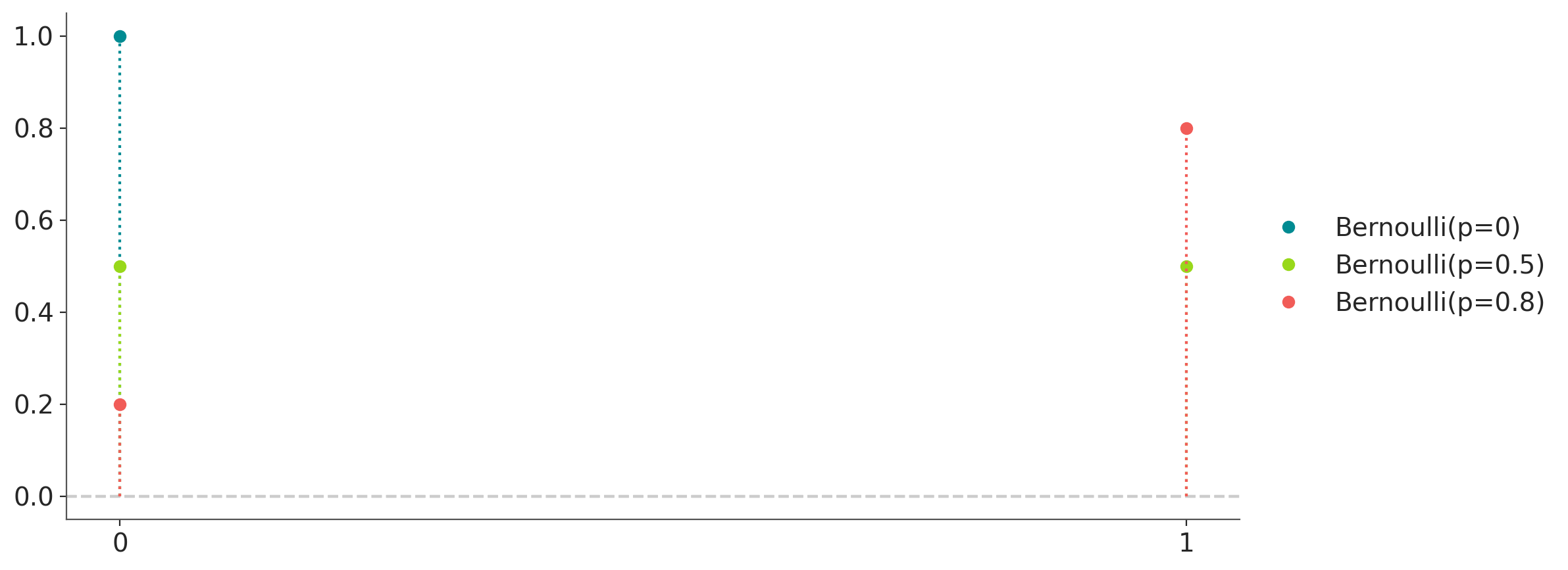
BetaBinomial probability distribution.

class preliz.distributions.betabinomial.BetaBinomial(alpha=None, beta=None, n=None)[source]#

Beta-binomial distribution.

Equivalent to binomial random variable with success probability drawn from a beta distribution.

The pmf of this distribution is

\[f(x \mid \alpha, \beta, n) = \binom{n}{x} \frac{B(x + \alpha, n - x + \beta)}{B(\alpha, \beta)}\]

(Source code, png, hires.png, pdf)

Support	$x \in \{0, 1, \ldots, n\}$
Mean	$n \dfrac{\alpha}{\alpha + \beta}$
Variance	$\dfrac{n \alpha \beta (\alpha+\beta+n)}{(\alpha+\beta)^2 (\alpha+\beta+1)}$

Parameters:

n (int) – Number of Bernoulli trials (n >= 0).
alpha (float) – alpha > 0.
beta (float) – beta > 0.

cdf(x)[source]#

Cumulative distribution function.

Parameters:: x (array_like) – Values on which to evaluate the cdf

entropy()[source]#: Entropy.

eti(mass=None, fmt='.2f')#

Equal-tailed interval containing mass.

Parameters:

mass (float) – Probability mass in the interval. Defaults to None,
used. (which results in the value of rcParams["stats.ci_prob"] being)
fmt (str) – fmt used to represent results using f-string fmt for floats. Default to “.2f” i.e. 2 digits after the decimal point. Use “none” for no format.

hdi(mass=None, fmt='.2f')#

Highest density interval containing mass.

Parameters:

mass (float) – Probability mass in the interval. Defaults to None,
used. (which results in the value of rcParams["stats.ci_prob"] being)
fmt (str) – fmt used to represent results using f-string fmt for floats. Default to “.2f” i.e. 2 digits after the decimal point. Use “none” for no format.

isf(x)#

Inverse survival function (inverse of sf).

Parameters:: x (array_like) – Values on which to evaluate the inverse of the sf

kurtosis()[source]#: Excess kurtosis.

lmoment1()[source]#: L-moment1 (mean).

lmoment2()[source]#: L-moment2 (l-scale).

lmoment3()[source]#: L-moment3 (l-skewness). This the ratio of L-moment3 to L-moment2.

lmoment4()[source]#: L-moment4 (l-kurtosis). This the ratio of L-moment4 to L-moment2.

lmoments(types='1234')#

Compute L-moments of the distribution.

Parameters:: types (str) – The type of moments to compute. Default is ‘1234’ where ‘1’ = L-moment1 (mean), ‘2’ = L-moment2 (l-scale), ‘3’ = L-moment3 (l-skewness), and ‘4’ = L-moment4 (l-kurtosis). To compute the standard deviation use ‘d’ Valid combinations are any subset of ‘1234’.

logcdf(x)#

Log cumulative distribution function.

Parameters:: x (array_like) – Values on which to evaluate the logcdf

logpdf(x)[source]#

Log probability density/mass function.

Parameters:: x (array_like) – Values on which to evaluate the logpdf

logsf(x)#

Log survival function log(1 - cdf).

Parameters:: x (array_like) – Values on which to evaluate the logsf

mean()[source]#: Mean.

median()[source]#: Median.

mode()[source]#: Mode.

moments(types='mvsk')#

Compute moments of the distribution.

It can also return the standard deviation

Parameters:: types (str) – The type of moments to compute. Default is ‘mvsk’ where ‘m’ = mean, ‘v’ = variance, ‘s’ = skewness, and ‘k’ = kurtosis. To compute the standard deviation use ‘d’ Valid combinations are any subset of ‘mvdsk’.

pdf(x)[source]#

Probability density/mass function.

Parameters:: x (array_like) – Values on which to evaluate the pdf

plot_cdf(moments=None, pointinterval=False, interval=None, levels=None, support='restricted', legend='legend', figsize=None, ax=None, **kwargs)#

Plot the cumulative distribution function.

Parameters:

moments (str) – Compute moments. Use any combination of the strings m, d, v, s or k for the mean (μ), standard deviation (σ), variance (σ²), skew (γ) or kurtosis (κ) respectively. Other strings will be ignored. Defaults to None.
pointinterval (bool) – Whether to include a plot of the quantiles. Defaults to False. If True the default is to plot the median and two interquantiles ranges.
interval (str) – Type of interval. Available options are highest density interval “hdi” (default), equal tailed interval “eti” or intervals defined by arbitrary “quantiles”. Defaults to the value in rcParams[“stats.ci_kind”].
levels (list) – Mass of the intervals. For hdi or eti the number of elements should be 2 or 1. For quantiles the number of elements should be 5, 3, 1 or 0 (in this last case nothing will be plotted).
support (str:) – If full use the finite end-points to set the limits of the plot. For unbounded end-points or if restricted use the 0.001 and 0.999 quantiles to set the limits.
legend (str) – Whether to include a string with the distribution and its parameter as a "legend" a "title" or not include them None.
figsize (tuple) – Size of the figure
ax (matplotlib axes)
kwargs (keyword arguments) – Additional keyword arguments passed to matplotlib plot function. For example, color, alpha, linewidth, etc.

plot_interactive(kind='pdf', xy_lim='both', pointinterval=True, interval=None, levels=None, figsize=None)#

Interactive exploration of distributions parameters.

Parameters:

kind (str:) – Type of plot. Available options are pdf, cdf and ppf.
xy_lim (str or tuple) – Set the limits of the x-axis and/or y-axis. Defaults to “both”, the limits of both axis are fixed. Use “auto” for automatic rescaling of x-axis and y-axis. Or set them manually by passing a tuple of 4 elements, the first two for x-axis, the last two for y-axis. The tuple can have None.
pointinterval (bool) – Whether to include a plot of the quantiles. Defaults to False. If True the default is to plot the median and two interquantiles ranges.
interval (str) – Type of interval. Available options are highest density interval “hdi” (default), equal tailed interval “eti” or intervals defined by arbitrary “quantiles”. Defaults to the value in rcParams[“stats.ci_kind”].
levels (list) – Mass of the intervals. For hdi or eti the number of elements should be 2 or 1. For quantiles the number of elements should be 5, 3, 1 or 0 (in this last case nothing will be plotted).
figsize (tuple) – Size of the figure

plot_isf(moments=None, pointinterval=False, interval=None, levels=None, legend='legend', figsize=None, ax=None, **kwargs)#

Plot the inverse survival function.

Parameters:

moments (str) – Compute moments. Use any combination of the strings m, d, v, s or k for the mean (μ), standard deviation (σ), variance (σ²), skew (γ) or kurtosis (κ) respectively. Other strings will be ignored. Defaults to None.
pointinterval (bool) – Whether to include a plot of the quantiles. Defaults to False. If True the default is to plot the median and two interquantiles ranges.
interval (str) – Type of interval. Available options are highest density interval “hdi” (default), equal tailed interval “eti” or intervals defined by arbitrary “quantiles”. Defaults to the value in rcParams[“stats.ci_kind”].
levels (list) – Mass of the intervals. For hdi or eti the number of elements should be 2 or 1. For quantiles the number of elements should be 5, 3, 1 or 0 (in this last case nothing will be plotted).
legend (str) – Whether to include a string with the distribution and its parameter as a "legend" a "title" or not include them None.
figsize (tuple) – Size of the figure
ax (matplotlib axes)

plot_pdf(moments=None, pointinterval=False, interval=None, levels=None, support='restricted', baseline=True, legend='legend', figsize=None, ax=None, **kwargs)#

Plot the pdf (continuous) or pmf (discrete).

Parameters:

moments (str) – Compute moments. Use any combination of the strings m, d, v, s or k for the mean (μ), standard deviation (σ), variance (σ²), skew (γ) or kurtosis (κ) respectively. Other strings will be ignored. Defaults to None.
pointinterval (bool) – Whether to include a plot of the quantiles. Defaults to False. If True the default is to plot the median and two interquantiles ranges.
interval (str) – Type of interval. Available options are highest density interval “hdi” (default), equal tailed interval “eti” or intervals defined by arbitrary “quantiles”. Defaults to the value in rcParams[“stats.ci_kind”].
levels (list) – Mass of the intervals. For hdi or eti the number of elements should be 2 or 1. For quantiles the number of elements should be 5, 3, 1 or 0 (in this last case nothing will be plotted).
support (str:) – If full use the finite end-points to set the limits of the plot. For unbounded end-points or if restricted use the 0.001 and 0.999 quantiles to set the limits.
baseline (bool) – Whether to include a horizontal line at y=0.
legend (str) – Whether to include a string with the distribution and its parameter as a "legend" a "title" or not include them None.
figsize (tuple) – Size of the figure
ax (matplotlib axes)
kwargs (keyword arguments) – Additional keyword arguments passed to matplotlib plot function. For example, color, alpha, linewidth, etc.

plot_ppf(moments=None, pointinterval=False, interval=None, levels=None, legend='legend', figsize=None, ax=None, **kwargs)#

Plot the quantile function.

Parameters:

moments (str) – Compute moments. Use any combination of the strings m, d, v, s or k for the mean (μ), standard deviation (σ), variance (σ²), skew (γ) or kurtosis (κ) respectively. Other strings will be ignored. Defaults to None.
pointinterval (bool) – Whether to include a plot of the quantiles. Defaults to False. If True the default is to plot the median and two interquantiles ranges.
interval (str) – Type of interval. Available options are highest density interval “hdi” (default), equal tailed interval “eti” or intervals defined by arbitrary “quantiles”. Defaults to the value in rcParams[“stats.ci_kind”].
levels (list) – Mass of the intervals. For hdi or eti the number of elements should be 2 or 1. For quantiles the number of elements should be 5, 3, 1 or 0 (in this last case nothing will be plotted).
legend (str) – Whether to include a string with the distribution and its parameter as a "legend" a "title" or not include them None.
figsize (tuple) – Size of the figure
ax (matplotlib axes)

plot_sf(moments=None, pointinterval=False, interval=None, levels=None, support='restricted', legend='legend', figsize=None, ax=None, **kwargs)#

Plot the survival distribution function (1 - CDF).

Parameters:

moments (str) – Compute moments. Use any combination of the strings m, d, v, s or k for the mean (μ), standard deviation (σ), variance (σ²), skew (γ) or kurtosis (κ) respectively. Other strings will be ignored. Defaults to None.
pointinterval (bool) – Whether to include a plot of the quantiles. Defaults to False. If True the default is to plot the median and two interquantiles ranges.
interval (str) – Type of interval. Available options are highest density interval “hdi” (default), equal tailed interval “eti” or intervals defined by arbitrary “quantiles”. Defaults to the value in rcParams[“stats.ci_kind”].
levels (list) – Mass of the intervals. For hdi or eti the number of elements should be 2 or 1. For quantiles the number of elements should be 5, 3, 1 or 0 (in this last case nothing will be plotted).
support (str:) – If full use the finite end-points to set the limits of the plot. For unbounded end-points or if restricted use the 0.001 and 0.999 quantiles to set the limits.
legend (str) – Whether to include a string with the distribution and its parameter as a "legend" a "title" or not include them None.
figsize (tuple) – Size of the figure
ax (matplotlib axes)
kwargs (keyword arguments) – Additional keyword arguments passed to matplotlib plot function. For example, color, alpha, linewidth, etc.

ppf(q)[source]#

Percent point function (inverse of cdf).

Parameters:: x (array_like) – Values on which to evaluate the inverse of the cdf

rvs(size=None, random_state=None)[source]#

Random sample.

Parameters:

size (int or tuple of ints, optional) – Defining number of random variates. Defaults to 1.
random_state ({None, int, numpy.random.Generator, numpy.random.RandomState}) – Defaults to None

sf(x)#

Survival function (1 - cdf).

Parameters:: x (array_like) – Values on which to evaluate the sf

skewness()[source]#: Skewness.

std()[source]#: Standard deviation.

summary(mass=None, interval=None, fmt='.2f')#

Namedtuple with the mean, median, sd, and lower and upper bounds.

Parameters:

mass (float) – Probability mass for the equal-tailed interval. Defaults to None,
used. (which results in the value of rcParams["stats.ci_prob"] being)
interval (str or list-like) – Type of interval. Available options are highest density interval “hdi”, equal tailed interval “eti” or arbitrary interval defined by a list-like object with a pair of values. Defaults to the value in rcParams[“stats.ci_kind”].
fmt (str) – fmt used to represent results using f-string fmt for floats. Default to “.2f” i.e. 2 digits after the decimal point.

to_bambi(**kwargs)#

Convert the PreliZ distribution to a Bambi Prior.

kwargsPyMC distributions properties: kwargs are used to specify properties such as shape or dims

Return type:: Bambi Prior

to_pymc(name=None, **kwargs)#

Convert the PreliZ distribution to a PyMC distribution.

namestr: Name of PyMC distribution. Needed if inside Model context
kwargsPyMC distributions properties: kwargs are used to specify properties such as shape or dims

Return type:: PyMC distribution

var()[source]#: Variance.

xvals(support, n_points=None)#

Provide x values in the support of the distribution.

This is useful for example when plotting.

Parameters:

support (str) – Available options are “full” or “restricted”. If “full” the values will cover the entire support of the distribution if the boundary is finite, or the quantiles 0.0001 or 0.9999, if infinite. If “restricted” the values will cover the quantile 0.0001 to 0.9999.
n_points (int) – Number of values to return. Defaults to 1000 for continuous distributions and 200 for discrete ones. For discrete distributions the returned values may be fewer than n_points if the actual number of discrete values in the support of the distribution is smaller than n_points.

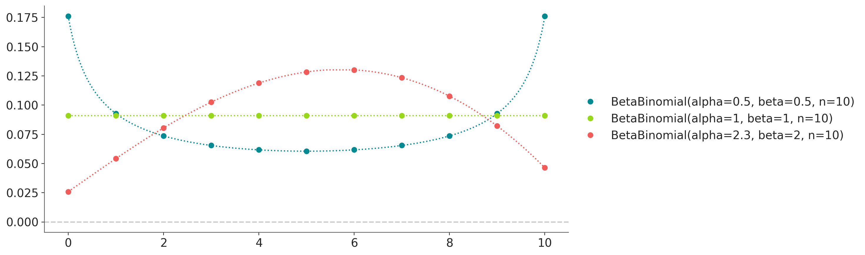
class preliz.distributions.binomial.Binomial(n=None, p=None)[source]#

Binomial distribution.

The discrete probability distribution of the number of successes in a sequence of n independent yes/no experiments, each of which yields success with probability p.

The pmf of this distribution is

\[f(x \mid n, p) = \binom{n}{x} p^x (1-p)^{n-x}\]

(Source code, png, hires.png, pdf)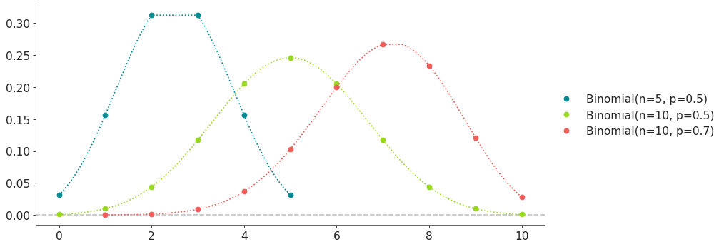

Support	$x \in \{0, 1, \ldots, n\}$
Mean	$n p$
Variance	$n p (1 - p)$

Parameters:

n (int) – Number of Bernoulli trials (n >= 0).
p (float) – Probability of success in each trial (0 < p < 1).

cdf(x)[source]#

Cumulative distribution function.

Parameters:: x (array_like) – Values on which to evaluate the cdf

entropy()[source]#: Entropy.

eti(mass=None, fmt='.2f')#

Equal-tailed interval containing mass.

Parameters:

mass (float) – Probability mass in the interval. Defaults to None,
used. (which results in the value of rcParams["stats.ci_prob"] being)
fmt (str) – fmt used to represent results using f-string fmt for floats. Default to “.2f” i.e. 2 digits after the decimal point. Use “none” for no format.

hdi(mass=None, fmt='.2f')#

Highest density interval containing mass.

Parameters:

mass (float) – Probability mass in the interval. Defaults to None,
used. (which results in the value of rcParams["stats.ci_prob"] being)
fmt (str) – fmt used to represent results using f-string fmt for floats. Default to “.2f” i.e. 2 digits after the decimal point. Use “none” for no format.

isf(x)#

Inverse survival function (inverse of sf).

Parameters:: x (array_like) – Values on which to evaluate the inverse of the sf

kurtosis()[source]#: Excess kurtosis.

lmoment1()[source]#: L-moment1 (mean).

lmoment2()[source]#: L-moment2 (l-scale).

lmoment3()[source]#: L-moment3 (l-skewness). This the ratio of L-moment3 to L-moment2.

lmoment4()[source]#: L-moment4 (l-kurtosis). This the ratio of L-moment4 to L-moment2.

lmoments(types='1234')#

Compute L-moments of the distribution.

Parameters:: types (str) – The type of moments to compute. Default is ‘1234’ where ‘1’ = L-moment1 (mean), ‘2’ = L-moment2 (l-scale), ‘3’ = L-moment3 (l-skewness), and ‘4’ = L-moment4 (l-kurtosis). To compute the standard deviation use ‘d’ Valid combinations are any subset of ‘1234’.

logcdf(x)#

Log cumulative distribution function.

Parameters:: x (array_like) – Values on which to evaluate the logcdf

logpdf(x)[source]#

Log probability density/mass function.

Parameters:: x (array_like) – Values on which to evaluate the logpdf

logsf(x)#

Log survival function log(1 - cdf).

Parameters:: x (array_like) – Values on which to evaluate the logsf

mean()[source]#: Mean.

median()[source]#: Median.

mode()[source]#: Mode.

moments(types='mvsk')#

Compute moments of the distribution.

It can also return the standard deviation

Parameters:: types (str) – The type of moments to compute. Default is ‘mvsk’ where ‘m’ = mean, ‘v’ = variance, ‘s’ = skewness, and ‘k’ = kurtosis. To compute the standard deviation use ‘d’ Valid combinations are any subset of ‘mvdsk’.

pdf(x)[source]#

Probability density/mass function.

Parameters:: x (array_like) – Values on which to evaluate the pdf

plot_cdf(moments=None, pointinterval=False, interval=None, levels=None, support='restricted', legend='legend', figsize=None, ax=None, **kwargs)#

Plot the cumulative distribution function.

Parameters:

moments (str) – Compute moments. Use any combination of the strings m, d, v, s or k for the mean (μ), standard deviation (σ), variance (σ²), skew (γ) or kurtosis (κ) respectively. Other strings will be ignored. Defaults to None.
pointinterval (bool) – Whether to include a plot of the quantiles. Defaults to False. If True the default is to plot the median and two interquantiles ranges.
interval (str) – Type of interval. Available options are highest density interval “hdi” (default), equal tailed interval “eti” or intervals defined by arbitrary “quantiles”. Defaults to the value in rcParams[“stats.ci_kind”].
levels (list) – Mass of the intervals. For hdi or eti the number of elements should be 2 or 1. For quantiles the number of elements should be 5, 3, 1 or 0 (in this last case nothing will be plotted).
support (str:) – If full use the finite end-points to set the limits of the plot. For unbounded end-points or if restricted use the 0.001 and 0.999 quantiles to set the limits.
legend (str) – Whether to include a string with the distribution and its parameter as a "legend" a "title" or not include them None.
figsize (tuple) – Size of the figure
ax (matplotlib axes)
kwargs (keyword arguments) – Additional keyword arguments passed to matplotlib plot function. For example, color, alpha, linewidth, etc.

plot_interactive(kind='pdf', xy_lim='both', pointinterval=True, interval=None, levels=None, figsize=None)#

Interactive exploration of distributions parameters.

Parameters:

kind (str:) – Type of plot. Available options are pdf, cdf and ppf.
xy_lim (str or tuple) – Set the limits of the x-axis and/or y-axis. Defaults to “both”, the limits of both axis are fixed. Use “auto” for automatic rescaling of x-axis and y-axis. Or set them manually by passing a tuple of 4 elements, the first two for x-axis, the last two for y-axis. The tuple can have None.
pointinterval (bool) – Whether to include a plot of the quantiles. Defaults to False. If True the default is to plot the median and two interquantiles ranges.
interval (str) – Type of interval. Available options are highest density interval “hdi” (default), equal tailed interval “eti” or intervals defined by arbitrary “quantiles”. Defaults to the value in rcParams[“stats.ci_kind”].
levels (list) – Mass of the intervals. For hdi or eti the number of elements should be 2 or 1. For quantiles the number of elements should be 5, 3, 1 or 0 (in this last case nothing will be plotted).
figsize (tuple) – Size of the figure

plot_isf(moments=None, pointinterval=False, interval=None, levels=None, legend='legend', figsize=None, ax=None, **kwargs)#

Plot the inverse survival function.

Parameters:

moments (str) – Compute moments. Use any combination of the strings m, d, v, s or k for the mean (μ), standard deviation (σ), variance (σ²), skew (γ) or kurtosis (κ) respectively. Other strings will be ignored. Defaults to None.
pointinterval (bool) – Whether to include a plot of the quantiles. Defaults to False. If True the default is to plot the median and two interquantiles ranges.
interval (str) – Type of interval. Available options are highest density interval “hdi” (default), equal tailed interval “eti” or intervals defined by arbitrary “quantiles”. Defaults to the value in rcParams[“stats.ci_kind”].
levels (list) – Mass of the intervals. For hdi or eti the number of elements should be 2 or 1. For quantiles the number of elements should be 5, 3, 1 or 0 (in this last case nothing will be plotted).
legend (str) – Whether to include a string with the distribution and its parameter as a "legend" a "title" or not include them None.
figsize (tuple) – Size of the figure
ax (matplotlib axes)

plot_pdf(moments=None, pointinterval=False, interval=None, levels=None, support='restricted', baseline=True, legend='legend', figsize=None, ax=None, **kwargs)#

Plot the pdf (continuous) or pmf (discrete).

Parameters:

moments (str) – Compute moments. Use any combination of the strings m, d, v, s or k for the mean (μ), standard deviation (σ), variance (σ²), skew (γ) or kurtosis (κ) respectively. Other strings will be ignored. Defaults to None.
pointinterval (bool) – Whether to include a plot of the quantiles. Defaults to False. If True the default is to plot the median and two interquantiles ranges.
interval (str) – Type of interval. Available options are highest density interval “hdi” (default), equal tailed interval “eti” or intervals defined by arbitrary “quantiles”. Defaults to the value in rcParams[“stats.ci_kind”].
levels (list) – Mass of the intervals. For hdi or eti the number of elements should be 2 or 1. For quantiles the number of elements should be 5, 3, 1 or 0 (in this last case nothing will be plotted).
support (str:) – If full use the finite end-points to set the limits of the plot. For unbounded end-points or if restricted use the 0.001 and 0.999 quantiles to set the limits.
baseline (bool) – Whether to include a horizontal line at y=0.
legend (str) – Whether to include a string with the distribution and its parameter as a "legend" a "title" or not include them None.
figsize (tuple) – Size of the figure
ax (matplotlib axes)
kwargs (keyword arguments) – Additional keyword arguments passed to matplotlib plot function. For example, color, alpha, linewidth, etc.

plot_ppf(moments=None, pointinterval=False, interval=None, levels=None, legend='legend', figsize=None, ax=None, **kwargs)#

Plot the quantile function.

Parameters:

moments (str) – Compute moments. Use any combination of the strings m, d, v, s or k for the mean (μ), standard deviation (σ), variance (σ²), skew (γ) or kurtosis (κ) respectively. Other strings will be ignored. Defaults to None.
pointinterval (bool) – Whether to include a plot of the quantiles. Defaults to False. If True the default is to plot the median and two interquantiles ranges.
interval (str) – Type of interval. Available options are highest density interval “hdi” (default), equal tailed interval “eti” or intervals defined by arbitrary “quantiles”. Defaults to the value in rcParams[“stats.ci_kind”].
levels (list) – Mass of the intervals. For hdi or eti the number of elements should be 2 or 1. For quantiles the number of elements should be 5, 3, 1 or 0 (in this last case nothing will be plotted).
legend (str) – Whether to include a string with the distribution and its parameter as a "legend" a "title" or not include them None.
figsize (tuple) – Size of the figure
ax (matplotlib axes)

plot_sf(moments=None, pointinterval=False, interval=None, levels=None, support='restricted', legend='legend', figsize=None, ax=None, **kwargs)#

Plot the survival distribution function (1 - CDF).

Parameters:

moments (str) – Compute moments. Use any combination of the strings m, d, v, s or k for the mean (μ), standard deviation (σ), variance (σ²), skew (γ) or kurtosis (κ) respectively. Other strings will be ignored. Defaults to None.
pointinterval (bool) – Whether to include a plot of the quantiles. Defaults to False. If True the default is to plot the median and two interquantiles ranges.
interval (str) – Type of interval. Available options are highest density interval “hdi” (default), equal tailed interval “eti” or intervals defined by arbitrary “quantiles”. Defaults to the value in rcParams[“stats.ci_kind”].
levels (list) – Mass of the intervals. For hdi or eti the number of elements should be 2 or 1. For quantiles the number of elements should be 5, 3, 1 or 0 (in this last case nothing will be plotted).
support (str:) – If full use the finite end-points to set the limits of the plot. For unbounded end-points or if restricted use the 0.001 and 0.999 quantiles to set the limits.
legend (str) – Whether to include a string with the distribution and its parameter as a "legend" a "title" or not include them None.
figsize (tuple) – Size of the figure
ax (matplotlib axes)
kwargs (keyword arguments) – Additional keyword arguments passed to matplotlib plot function. For example, color, alpha, linewidth, etc.

ppf(q)[source]#

Percent point function (inverse of cdf).

Parameters:: x (array_like) – Values on which to evaluate the inverse of the cdf

rvs(size=None, random_state=None)[source]#

Random sample.

Parameters:

size (int or tuple of ints, optional) – Defining number of random variates. Defaults to 1.
random_state ({None, int, numpy.random.Generator, numpy.random.RandomState}) – Defaults to None

sf(x)#

Survival function (1 - cdf).

Parameters:: x (array_like) – Values on which to evaluate the sf

skewness()[source]#: Skewness.

std()[source]#: Standard deviation.

summary(mass=None, interval=None, fmt='.2f')#

Namedtuple with the mean, median, sd, and lower and upper bounds.

Parameters:

mass (float) – Probability mass for the equal-tailed interval. Defaults to None,
used. (which results in the value of rcParams["stats.ci_prob"] being)
interval (str or list-like) – Type of interval. Available options are highest density interval “hdi”, equal tailed interval “eti” or arbitrary interval defined by a list-like object with a pair of values. Defaults to the value in rcParams[“stats.ci_kind”].
fmt (str) – fmt used to represent results using f-string fmt for floats. Default to “.2f” i.e. 2 digits after the decimal point.

to_bambi(**kwargs)#

Convert the PreliZ distribution to a Bambi Prior.

kwargsPyMC distributions properties: kwargs are used to specify properties such as shape or dims

Return type:: Bambi Prior

to_pymc(name=None, **kwargs)#

Convert the PreliZ distribution to a PyMC distribution.

namestr: Name of PyMC distribution. Needed if inside Model context
kwargsPyMC distributions properties: kwargs are used to specify properties such as shape or dims

Return type:: PyMC distribution

var()[source]#: Variance.

xvals(support, n_points=None)#

Provide x values in the support of the distribution.

This is useful for example when plotting.

Parameters:

support (str) – Available options are “full” or “restricted”. If “full” the values will cover the entire support of the distribution if the boundary is finite, or the quantiles 0.0001 or 0.9999, if infinite. If “restricted” the values will cover the quantile 0.0001 to 0.9999.
n_points (int) – Number of values to return. Defaults to 1000 for continuous distributions and 200 for discrete ones. For discrete distributions the returned values may be fewer than n_points if the actual number of discrete values in the support of the distribution is smaller than n_points.

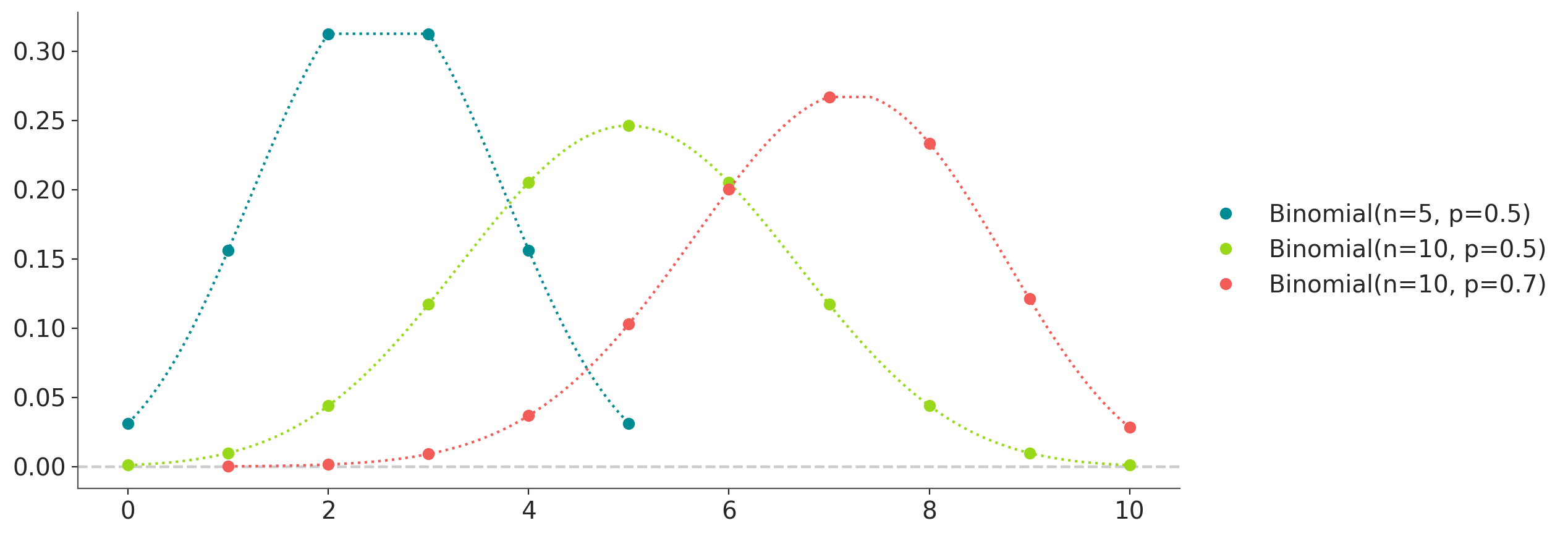
class preliz.distributions.categorical.Categorical(p=None, logit_p=None)[source]#

Categorical distribution.

The most general discrete distribution. The pmf of this distribution is

\[f(x \mid p) = p_x\]

(Source code, png, hires.png, pdf)

Support

$x \in \{0, 1, \ldots, |p|-1\}$

Parameters:

p (array of floats) – p > 0 and the elements of p must sum to 1.
logit_p (float) – Alternative log odds for the probability of success.

cdf(x)[source]#

Cumulative distribution function.

Parameters:: x (array_like) – Values on which to evaluate the cdf

entropy()[source]#: Entropy.

eti(mass=None, fmt='.2f')#

Equal-tailed interval containing mass.

Parameters:

mass (float) – Probability mass in the interval. Defaults to None,
used. (which results in the value of rcParams["stats.ci_prob"] being)
fmt (str) – fmt used to represent results using f-string fmt for floats. Default to “.2f” i.e. 2 digits after the decimal point. Use “none” for no format.

hdi(mass=None, fmt='.2f')#

Highest density interval containing mass.

Parameters:

mass (float) – Probability mass in the interval. Defaults to None,
used. (which results in the value of rcParams["stats.ci_prob"] being)
fmt (str) – fmt used to represent results using f-string fmt for floats. Default to “.2f” i.e. 2 digits after the decimal point. Use “none” for no format.

isf(x)#

Inverse survival function (inverse of sf).

Parameters:: x (array_like) – Values on which to evaluate the inverse of the sf

kurtosis()[source]#: Excess kurtosis.

lmoment1()#: L-moment1 (mean).

lmoment2()#: L-moment2 (l-scale).

lmoment3()#: L-moment3 (l-skewness). This the ratio of L-moment3 to L-moment2.

lmoment4()#: L-moment4 (l-kurtosis). This the ratio of L-moment4 to L-moment2.

lmoments(types='1234')#

Compute L-moments of the distribution.

Parameters:: types (str) – The type of moments to compute. Default is ‘1234’ where ‘1’ = L-moment1 (mean), ‘2’ = L-moment2 (l-scale), ‘3’ = L-moment3 (l-skewness), and ‘4’ = L-moment4 (l-kurtosis). To compute the standard deviation use ‘d’ Valid combinations are any subset of ‘1234’.

logcdf(x)#

Log cumulative distribution function.

Parameters:: x (array_like) – Values on which to evaluate the logcdf

logpdf(x)[source]#

Log probability density/mass function.

Parameters:: x (array_like) – Values on which to evaluate the logpdf

logsf(x)#

Log survival function log(1 - cdf).

Parameters:: x (array_like) – Values on which to evaluate the logsf

mean()[source]#: Mean.

median()[source]#: Median.

mode()[source]#: Mode.

moments(types='mvsk')#

Compute moments of the distribution.

It can also return the standard deviation

Parameters:: types (str) – The type of moments to compute. Default is ‘mvsk’ where ‘m’ = mean, ‘v’ = variance, ‘s’ = skewness, and ‘k’ = kurtosis. To compute the standard deviation use ‘d’ Valid combinations are any subset of ‘mvdsk’.

pdf(x)[source]#

Probability density/mass function.

Parameters:: x (array_like) – Values on which to evaluate the pdf

plot_cdf(moments=None, pointinterval=False, interval=None, levels=None, support='restricted', legend='legend', figsize=None, ax=None, **kwargs)#

Plot the cumulative distribution function.

Parameters:

moments (str) – Compute moments. Use any combination of the strings m, d, v, s or k for the mean (μ), standard deviation (σ), variance (σ²), skew (γ) or kurtosis (κ) respectively. Other strings will be ignored. Defaults to None.
pointinterval (bool) – Whether to include a plot of the quantiles. Defaults to False. If True the default is to plot the median and two interquantiles ranges.
interval (str) – Type of interval. Available options are highest density interval “hdi” (default), equal tailed interval “eti” or intervals defined by arbitrary “quantiles”. Defaults to the value in rcParams[“stats.ci_kind”].
levels (list) – Mass of the intervals. For hdi or eti the number of elements should be 2 or 1. For quantiles the number of elements should be 5, 3, 1 or 0 (in this last case nothing will be plotted).
support (str:) – If full use the finite end-points to set the limits of the plot. For unbounded end-points or if restricted use the 0.001 and 0.999 quantiles to set the limits.
legend (str) – Whether to include a string with the distribution and its parameter as a "legend" a "title" or not include them None.
figsize (tuple) – Size of the figure
ax (matplotlib axes)
kwargs (keyword arguments) – Additional keyword arguments passed to matplotlib plot function. For example, color, alpha, linewidth, etc.

plot_interactive(kind='pdf', xy_lim='both', pointinterval=True, interval=None, levels=None, figsize=None)#

Interactive exploration of distributions parameters.

Parameters:

kind (str:) – Type of plot. Available options are pdf, cdf and ppf.
xy_lim (str or tuple) – Set the limits of the x-axis and/or y-axis. Defaults to “both”, the limits of both axis are fixed. Use “auto” for automatic rescaling of x-axis and y-axis. Or set them manually by passing a tuple of 4 elements, the first two for x-axis, the last two for y-axis. The tuple can have None.
pointinterval (bool) – Whether to include a plot of the quantiles. Defaults to False. If True the default is to plot the median and two interquantiles ranges.
interval (str) – Type of interval. Available options are highest density interval “hdi” (default), equal tailed interval “eti” or intervals defined by arbitrary “quantiles”. Defaults to the value in rcParams[“stats.ci_kind”].
levels (list) – Mass of the intervals. For hdi or eti the number of elements should be 2 or 1. For quantiles the number of elements should be 5, 3, 1 or 0 (in this last case nothing will be plotted).
figsize (tuple) – Size of the figure

plot_isf(moments=None, pointinterval=False, interval=None, levels=None, legend='legend', figsize=None, ax=None, **kwargs)#

Plot the inverse survival function.

Parameters:

moments (str) – Compute moments. Use any combination of the strings m, d, v, s or k for the mean (μ), standard deviation (σ), variance (σ²), skew (γ) or kurtosis (κ) respectively. Other strings will be ignored. Defaults to None.
pointinterval (bool) – Whether to include a plot of the quantiles. Defaults to False. If True the default is to plot the median and two interquantiles ranges.
interval (str) – Type of interval. Available options are highest density interval “hdi” (default), equal tailed interval “eti” or intervals defined by arbitrary “quantiles”. Defaults to the value in rcParams[“stats.ci_kind”].
levels (list) – Mass of the intervals. For hdi or eti the number of elements should be 2 or 1. For quantiles the number of elements should be 5, 3, 1 or 0 (in this last case nothing will be plotted).
legend (str) – Whether to include a string with the distribution and its parameter as a "legend" a "title" or not include them None.
figsize (tuple) – Size of the figure
ax (matplotlib axes)

plot_pdf(moments=None, pointinterval=False, interval=None, levels=None, support='restricted', baseline=True, legend='legend', figsize=None, ax=None, **kwargs)#

Plot the pdf (continuous) or pmf (discrete).

Parameters:

moments (str) – Compute moments. Use any combination of the strings m, d, v, s or k for the mean (μ), standard deviation (σ), variance (σ²), skew (γ) or kurtosis (κ) respectively. Other strings will be ignored. Defaults to None.
pointinterval (bool) – Whether to include a plot of the quantiles. Defaults to False. If True the default is to plot the median and two interquantiles ranges.
interval (str) – Type of interval. Available options are highest density interval “hdi” (default), equal tailed interval “eti” or intervals defined by arbitrary “quantiles”. Defaults to the value in rcParams[“stats.ci_kind”].
levels (list) – Mass of the intervals. For hdi or eti the number of elements should be 2 or 1. For quantiles the number of elements should be 5, 3, 1 or 0 (in this last case nothing will be plotted).
support (str:) – If full use the finite end-points to set the limits of the plot. For unbounded end-points or if restricted use the 0.001 and 0.999 quantiles to set the limits.
baseline (bool) – Whether to include a horizontal line at y=0.
legend (str) – Whether to include a string with the distribution and its parameter as a "legend" a "title" or not include them None.
figsize (tuple) – Size of the figure
ax (matplotlib axes)
kwargs (keyword arguments) – Additional keyword arguments passed to matplotlib plot function. For example, color, alpha, linewidth, etc.

plot_ppf(moments=None, pointinterval=False, interval=None, levels=None, legend='legend', figsize=None, ax=None, **kwargs)#

Plot the quantile function.

Parameters:

moments (str) – Compute moments. Use any combination of the strings m, d, v, s or k for the mean (μ), standard deviation (σ), variance (σ²), skew (γ) or kurtosis (κ) respectively. Other strings will be ignored. Defaults to None.
pointinterval (bool) – Whether to include a plot of the quantiles. Defaults to False. If True the default is to plot the median and two interquantiles ranges.
interval (str) – Type of interval. Available options are highest density interval “hdi” (default), equal tailed interval “eti” or intervals defined by arbitrary “quantiles”. Defaults to the value in rcParams[“stats.ci_kind”].
levels (list) – Mass of the intervals. For hdi or eti the number of elements should be 2 or 1. For quantiles the number of elements should be 5, 3, 1 or 0 (in this last case nothing will be plotted).
legend (str) – Whether to include a string with the distribution and its parameter as a "legend" a "title" or not include them None.
figsize (tuple) – Size of the figure
ax (matplotlib axes)

plot_sf(moments=None, pointinterval=False, interval=None, levels=None, support='restricted', legend='legend', figsize=None, ax=None, **kwargs)#

Plot the survival distribution function (1 - CDF).

Parameters:

moments (str) – Compute moments. Use any combination of the strings m, d, v, s or k for the mean (μ), standard deviation (σ), variance (σ²), skew (γ) or kurtosis (κ) respectively. Other strings will be ignored. Defaults to None.
pointinterval (bool) – Whether to include a plot of the quantiles. Defaults to False. If True the default is to plot the median and two interquantiles ranges.
interval (str) – Type of interval. Available options are highest density interval “hdi” (default), equal tailed interval “eti” or intervals defined by arbitrary “quantiles”. Defaults to the value in rcParams[“stats.ci_kind”].
levels (list) – Mass of the intervals. For hdi or eti the number of elements should be 2 or 1. For quantiles the number of elements should be 5, 3, 1 or 0 (in this last case nothing will be plotted).
support (str:) – If full use the finite end-points to set the limits of the plot. For unbounded end-points or if restricted use the 0.001 and 0.999 quantiles to set the limits.
legend (str) – Whether to include a string with the distribution and its parameter as a "legend" a "title" or not include them None.
figsize (tuple) – Size of the figure
ax (matplotlib axes)
kwargs (keyword arguments) – Additional keyword arguments passed to matplotlib plot function. For example, color, alpha, linewidth, etc.

ppf(q)[source]#

Percent point function (inverse of cdf).

Parameters:: x (array_like) – Values on which to evaluate the inverse of the cdf

rvs(size=None, random_state=None)[source]#

Random sample.

Parameters:

size (int or tuple of ints, optional) – Defining number of random variates. Defaults to 1.
random_state ({None, int, numpy.random.Generator, numpy.random.RandomState}) – Defaults to None

sf(x)#

Survival function (1 - cdf).

Parameters:: x (array_like) – Values on which to evaluate the sf

skewness()[source]#: Skewness.

std()[source]#: Standard deviation.

summary(mass=None, interval=None, fmt='.2f')#

Namedtuple with the mean, median, sd, and lower and upper bounds.

Parameters:

mass (float) – Probability mass for the equal-tailed interval. Defaults to None,
used. (which results in the value of rcParams["stats.ci_prob"] being)
interval (str or list-like) – Type of interval. Available options are highest density interval “hdi”, equal tailed interval “eti” or arbitrary interval defined by a list-like object with a pair of values. Defaults to the value in rcParams[“stats.ci_kind”].
fmt (str) – fmt used to represent results using f-string fmt for floats. Default to “.2f” i.e. 2 digits after the decimal point.

to_bambi(**kwargs)#

Convert the PreliZ distribution to a Bambi Prior.

kwargsPyMC distributions properties: kwargs are used to specify properties such as shape or dims

Return type:: Bambi Prior

to_pymc(name=None, **kwargs)#

Convert the PreliZ distribution to a PyMC distribution.

namestr: Name of PyMC distribution. Needed if inside Model context
kwargsPyMC distributions properties: kwargs are used to specify properties such as shape or dims

Return type:: PyMC distribution

var()[source]#: Variance.

xvals(support, n_points=None)#

Provide x values in the support of the distribution.

This is useful for example when plotting.

Parameters:

support (str) – Available options are “full” or “restricted”. If “full” the values will cover the entire support of the distribution if the boundary is finite, or the quantiles 0.0001 or 0.9999, if infinite. If “restricted” the values will cover the quantile 0.0001 to 0.9999.
n_points (int) – Number of values to return. Defaults to 1000 for continuous distributions and 200 for discrete ones. For discrete distributions the returned values may be fewer than n_points if the actual number of discrete values in the support of the distribution is smaller than n_points.

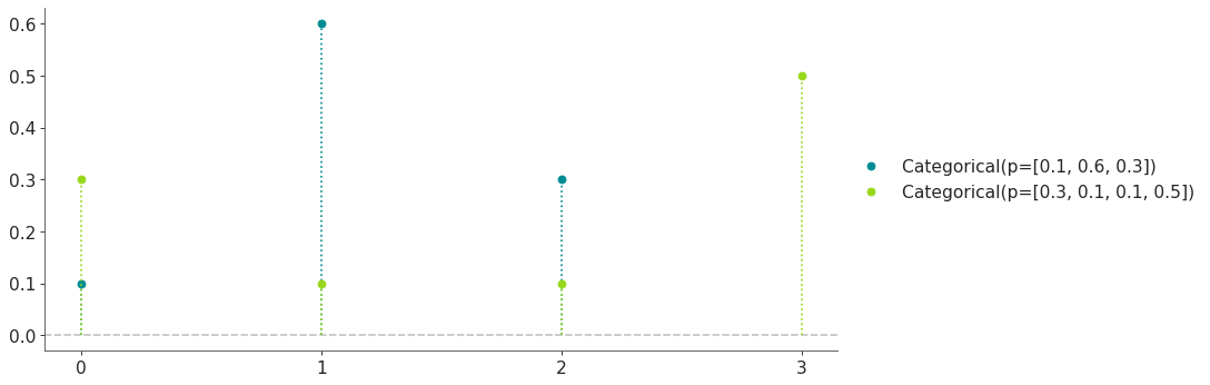
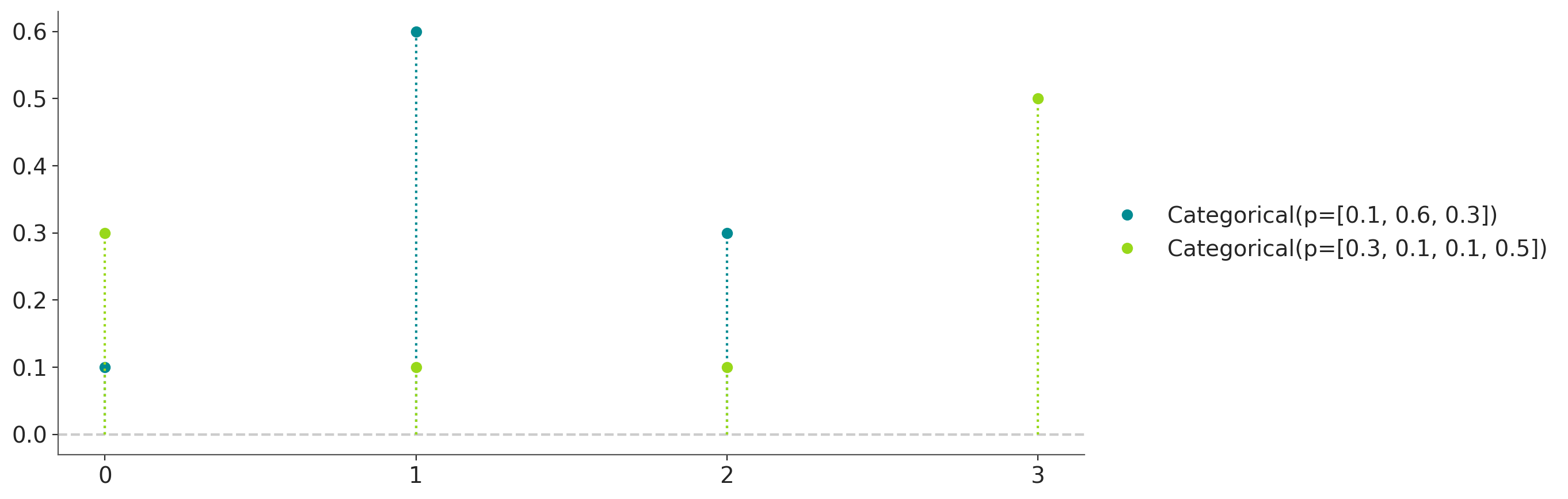
class preliz.distributions.discrete_uniform.DiscreteUniform(lower=None, upper=None)[source]#

Discrete Uniform distribution.

The pmf of this distribution is

\[f(x \mid lower, upper) = \frac{1}{upper-lower+1}\]

(Source code, png, hires.png, pdf)

Support	$x \in {lower, lower + 1, \ldots, upper}$
Mean	$\dfrac{lower + upper}{2}$
Variance	$\dfrac{(upper - lower + 1)^2 - 1}{12}$

Parameters:

lower (int) – Lower limit.
upper (int) – Upper limit (upper > lower).

cdf(x)[source]#

Cumulative distribution function.

Parameters:: x (array_like) – Values on which to evaluate the cdf

entropy()[source]#: Entropy.

eti(mass=None, fmt='.2f')#

Equal-tailed interval containing mass.

Parameters:

mass (float) – Probability mass in the interval. Defaults to None,
used. (which results in the value of rcParams["stats.ci_prob"] being)
fmt (str) – fmt used to represent results using f-string fmt for floats. Default to “.2f” i.e. 2 digits after the decimal point. Use “none” for no format.

hdi(mass=None, fmt='.2f')#

Highest density interval containing mass.

Parameters:

mass (float) – Probability mass in the interval. Defaults to None,
used. (which results in the value of rcParams["stats.ci_prob"] being)
fmt (str) – fmt used to represent results using f-string fmt for floats. Default to “.2f” i.e. 2 digits after the decimal point. Use “none” for no format.

isf(x)#

Inverse survival function (inverse of sf).

Parameters:: x (array_like) – Values on which to evaluate the inverse of the sf

kurtosis()[source]#: Excess kurtosis.

lmoment1()[source]#: L-moment1 (mean).

lmoment2()[source]#: L-moment2 (l-scale).

lmoment3()[source]#: L-moment3 (l-skewness). This the ratio of L-moment3 to L-moment2.

lmoment4()[source]#: L-moment4 (l-kurtosis). This the ratio of L-moment4 to L-moment2.

lmoments(types='1234')#

Compute L-moments of the distribution.

Parameters:: types (str) – The type of moments to compute. Default is ‘1234’ where ‘1’ = L-moment1 (mean), ‘2’ = L-moment2 (l-scale), ‘3’ = L-moment3 (l-skewness), and ‘4’ = L-moment4 (l-kurtosis). To compute the standard deviation use ‘d’ Valid combinations are any subset of ‘1234’.

logcdf(x)#

Log cumulative distribution function.

Parameters:: x (array_like) – Values on which to evaluate the logcdf

logpdf(x)[source]#

Log probability density/mass function.

Parameters:: x (array_like) – Values on which to evaluate the logpdf

logsf(x)#

Log survival function log(1 - cdf).

Parameters:: x (array_like) – Values on which to evaluate the logsf

mean()[source]#: Mean.

median()[source]#: Median.

mode()[source]#: Mode.

moments(types='mvsk')#

Compute moments of the distribution.

It can also return the standard deviation

Parameters:: types (str) – The type of moments to compute. Default is ‘mvsk’ where ‘m’ = mean, ‘v’ = variance, ‘s’ = skewness, and ‘k’ = kurtosis. To compute the standard deviation use ‘d’ Valid combinations are any subset of ‘mvdsk’.

pdf(x)[source]#

Probability density/mass function.

Parameters:: x (array_like) – Values on which to evaluate the pdf

plot_cdf(moments=None, pointinterval=False, interval=None, levels=None, support='restricted', legend='legend', figsize=None, ax=None, **kwargs)#

Plot the cumulative distribution function.

Parameters:

moments (str) – Compute moments. Use any combination of the strings m, d, v, s or k for the mean (μ), standard deviation (σ), variance (σ²), skew (γ) or kurtosis (κ) respectively. Other strings will be ignored. Defaults to None.
pointinterval (bool) – Whether to include a plot of the quantiles. Defaults to False. If True the default is to plot the median and two interquantiles ranges.
interval (str) – Type of interval. Available options are highest density interval “hdi” (default), equal tailed interval “eti” or intervals defined by arbitrary “quantiles”. Defaults to the value in rcParams[“stats.ci_kind”].
levels (list) – Mass of the intervals. For hdi or eti the number of elements should be 2 or 1. For quantiles the number of elements should be 5, 3, 1 or 0 (in this last case nothing will be plotted).
support (str:) – If full use the finite end-points to set the limits of the plot. For unbounded end-points or if restricted use the 0.001 and 0.999 quantiles to set the limits.
legend (str) – Whether to include a string with the distribution and its parameter as a "legend" a "title" or not include them None.
figsize (tuple) – Size of the figure
ax (matplotlib axes)
kwargs (keyword arguments) – Additional keyword arguments passed to matplotlib plot function. For example, color, alpha, linewidth, etc.

plot_interactive(kind='pdf', xy_lim='both', pointinterval=True, interval=None, levels=None, figsize=None)#

Interactive exploration of distributions parameters.

Parameters:

kind (str:) – Type of plot. Available options are pdf, cdf and ppf.
xy_lim (str or tuple) – Set the limits of the x-axis and/or y-axis. Defaults to “both”, the limits of both axis are fixed. Use “auto” for automatic rescaling of x-axis and y-axis. Or set them manually by passing a tuple of 4 elements, the first two for x-axis, the last two for y-axis. The tuple can have None.
pointinterval (bool) – Whether to include a plot of the quantiles. Defaults to False. If True the default is to plot the median and two interquantiles ranges.
interval (str) – Type of interval. Available options are highest density interval “hdi” (default), equal tailed interval “eti” or intervals defined by arbitrary “quantiles”. Defaults to the value in rcParams[“stats.ci_kind”].
levels (list) – Mass of the intervals. For hdi or eti the number of elements should be 2 or 1. For quantiles the number of elements should be 5, 3, 1 or 0 (in this last case nothing will be plotted).
figsize (tuple) – Size of the figure

plot_isf(moments=None, pointinterval=False, interval=None, levels=None, legend='legend', figsize=None, ax=None, **kwargs)#

Plot the inverse survival function.

Parameters:

moments (str) – Compute moments. Use any combination of the strings m, d, v, s or k for the mean (μ), standard deviation (σ), variance (σ²), skew (γ) or kurtosis (κ) respectively. Other strings will be ignored. Defaults to None.
pointinterval (bool) – Whether to include a plot of the quantiles. Defaults to False. If True the default is to plot the median and two interquantiles ranges.
interval (str) – Type of interval. Available options are highest density interval “hdi” (default), equal tailed interval “eti” or intervals defined by arbitrary “quantiles”. Defaults to the value in rcParams[“stats.ci_kind”].
levels (list) – Mass of the intervals. For hdi or eti the number of elements should be 2 or 1. For quantiles the number of elements should be 5, 3, 1 or 0 (in this last case nothing will be plotted).
legend (str) – Whether to include a string with the distribution and its parameter as a "legend" a "title" or not include them None.
figsize (tuple) – Size of the figure
ax (matplotlib axes)

plot_pdf(moments=None, pointinterval=False, interval=None, levels=None, support='restricted', baseline=True, legend='legend', figsize=None, ax=None, **kwargs)#

Plot the pdf (continuous) or pmf (discrete).

Parameters:

moments (str) – Compute moments. Use any combination of the strings m, d, v, s or k for the mean (μ), standard deviation (σ), variance (σ²), skew (γ) or kurtosis (κ) respectively. Other strings will be ignored. Defaults to None.
pointinterval (bool) – Whether to include a plot of the quantiles. Defaults to False. If True the default is to plot the median and two interquantiles ranges.
interval (str) – Type of interval. Available options are highest density interval “hdi” (default), equal tailed interval “eti” or intervals defined by arbitrary “quantiles”. Defaults to the value in rcParams[“stats.ci_kind”].
levels (list) – Mass of the intervals. For hdi or eti the number of elements should be 2 or 1. For quantiles the number of elements should be 5, 3, 1 or 0 (in this last case nothing will be plotted).
support (str:) – If full use the finite end-points to set the limits of the plot. For unbounded end-points or if restricted use the 0.001 and 0.999 quantiles to set the limits.
baseline (bool) – Whether to include a horizontal line at y=0.
legend (str) – Whether to include a string with the distribution and its parameter as a "legend" a "title" or not include them None.
figsize (tuple) – Size of the figure
ax (matplotlib axes)
kwargs (keyword arguments) – Additional keyword arguments passed to matplotlib plot function. For example, color, alpha, linewidth, etc.

plot_ppf(moments=None, pointinterval=False, interval=None, levels=None, legend='legend', figsize=None, ax=None, **kwargs)#

Plot the quantile function.

Parameters:

moments (str) – Compute moments. Use any combination of the strings m, d, v, s or k for the mean (μ), standard deviation (σ), variance (σ²), skew (γ) or kurtosis (κ) respectively. Other strings will be ignored. Defaults to None.
pointinterval (bool) – Whether to include a plot of the quantiles. Defaults to False. If True the default is to plot the median and two interquantiles ranges.
interval (str) – Type of interval. Available options are highest density interval “hdi” (default), equal tailed interval “eti” or intervals defined by arbitrary “quantiles”. Defaults to the value in rcParams[“stats.ci_kind”].
levels (list) – Mass of the intervals. For hdi or eti the number of elements should be 2 or 1. For quantiles the number of elements should be 5, 3, 1 or 0 (in this last case nothing will be plotted).
legend (str) – Whether to include a string with the distribution and its parameter as a "legend" a "title" or not include them None.
figsize (tuple) – Size of the figure
ax (matplotlib axes)

plot_sf(moments=None, pointinterval=False, interval=None, levels=None, support='restricted', legend='legend', figsize=None, ax=None, **kwargs)#

Plot the survival distribution function (1 - CDF).

Parameters:

moments (str) – Compute moments. Use any combination of the strings m, d, v, s or k for the mean (μ), standard deviation (σ), variance (σ²), skew (γ) or kurtosis (κ) respectively. Other strings will be ignored. Defaults to None.
pointinterval (bool) – Whether to include a plot of the quantiles. Defaults to False. If True the default is to plot the median and two interquantiles ranges.
interval (str) – Type of interval. Available options are highest density interval “hdi” (default), equal tailed interval “eti” or intervals defined by arbitrary “quantiles”. Defaults to the value in rcParams[“stats.ci_kind”].
levels (list) – Mass of the intervals. For hdi or eti the number of elements should be 2 or 1. For quantiles the number of elements should be 5, 3, 1 or 0 (in this last case nothing will be plotted).
support (str:) – If full use the finite end-points to set the limits of the plot. For unbounded end-points or if restricted use the 0.001 and 0.999 quantiles to set the limits.
legend (str) – Whether to include a string with the distribution and its parameter as a "legend" a "title" or not include them None.
figsize (tuple) – Size of the figure
ax (matplotlib axes)
kwargs (keyword arguments) – Additional keyword arguments passed to matplotlib plot function. For example, color, alpha, linewidth, etc.

ppf(q)[source]#

Percent point function (inverse of cdf).

Parameters:: x (array_like) – Values on which to evaluate the inverse of the cdf

rvs(size=None, random_state=None)[source]#

Random sample.

Parameters:

size (int or tuple of ints, optional) – Defining number of random variates. Defaults to 1.
random_state ({None, int, numpy.random.Generator, numpy.random.RandomState}) – Defaults to None

sf(x)#

Survival function (1 - cdf).

Parameters:: x (array_like) – Values on which to evaluate the sf

skewness()[source]#: Skewness.

std()[source]#: Standard deviation.

summary(mass=None, interval=None, fmt='.2f')#

Namedtuple with the mean, median, sd, and lower and upper bounds.

Parameters:

mass (float) – Probability mass for the equal-tailed interval. Defaults to None,
used. (which results in the value of rcParams["stats.ci_prob"] being)
interval (str or list-like) – Type of interval. Available options are highest density interval “hdi”, equal tailed interval “eti” or arbitrary interval defined by a list-like object with a pair of values. Defaults to the value in rcParams[“stats.ci_kind”].
fmt (str) – fmt used to represent results using f-string fmt for floats. Default to “.2f” i.e. 2 digits after the decimal point.

to_bambi(**kwargs)#

Convert the PreliZ distribution to a Bambi Prior.

kwargsPyMC distributions properties: kwargs are used to specify properties such as shape or dims

Return type:: Bambi Prior

to_pymc(name=None, **kwargs)#

Convert the PreliZ distribution to a PyMC distribution.

namestr: Name of PyMC distribution. Needed if inside Model context
kwargsPyMC distributions properties: kwargs are used to specify properties such as shape or dims

Return type:: PyMC distribution

var()[source]#: Variance.

xvals(support, n_points=None)#

Provide x values in the support of the distribution.

This is useful for example when plotting.

Parameters:

support (str) – Available options are “full” or “restricted”. If “full” the values will cover the entire support of the distribution if the boundary is finite, or the quantiles 0.0001 or 0.9999, if infinite. If “restricted” the values will cover the quantile 0.0001 to 0.9999.
n_points (int) – Number of values to return. Defaults to 1000 for continuous distributions and 200 for discrete ones. For discrete distributions the returned values may be fewer than n_points if the actual number of discrete values in the support of the distribution is smaller than n_points.

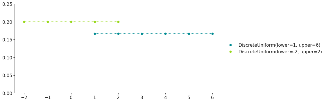
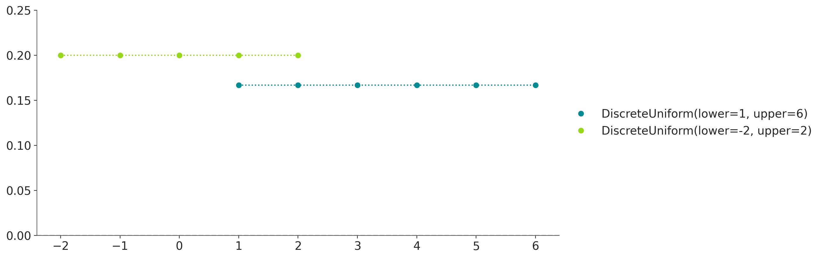
class preliz.distributions.discrete_weibull.DiscreteWeibull(q=None, beta=None)[source]#

Discrete Weibull distribution.

The pmf of this distribution is

\[f(x \mid q, \beta) = q^{x^{\beta}} - q^{(x+1)^{\beta}}\]

(Source code, png, hires.png, pdf)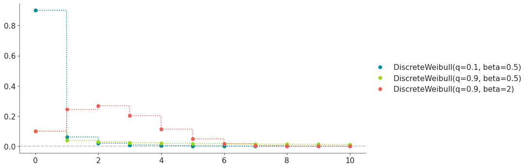

Support	$x \in \mathbb{N}_0$
Mean	$\mu = \sum_{x = 1}^{\infty} q^{x^{\beta}}$
Variance	$2 \sum_{x = 1}^{\infty} x q^{x^{\beta}} - \mu - \mu^2$

Parameters:

q (float) – Shape parameter (0 < q < 1).
beta (float) – Shape parameter (beta > 0).

cdf(x)[source]#

Cumulative distribution function.

Parameters:: x (array_like) – Values on which to evaluate the cdf

entropy()[source]#: Entropy.

eti(mass=None, fmt='.2f')#

Equal-tailed interval containing mass.

Parameters:

mass (float) – Probability mass in the interval. Defaults to None,
used. (which results in the value of rcParams["stats.ci_prob"] being)
fmt (str) – fmt used to represent results using f-string fmt for floats. Default to “.2f” i.e. 2 digits after the decimal point. Use “none” for no format.

hdi(mass=None, fmt='.2f')#

Highest density interval containing mass.

Parameters:

mass (float) – Probability mass in the interval. Defaults to None,
used. (which results in the value of rcParams["stats.ci_prob"] being)
fmt (str) – fmt used to represent results using f-string fmt for floats. Default to “.2f” i.e. 2 digits after the decimal point. Use “none” for no format.

isf(x)#

Inverse survival function (inverse of sf).

Parameters:: x (array_like) – Values on which to evaluate the inverse of the sf

kurtosis()[source]#: Excess kurtosis.

lmoment1()#: L-moment1 (mean).

lmoment2()#: L-moment2 (l-scale).

lmoment3()#: L-moment3 (l-skewness). This the ratio of L-moment3 to L-moment2.

lmoment4()#: L-moment4 (l-kurtosis). This the ratio of L-moment4 to L-moment2.

lmoments(types='1234')#

Compute L-moments of the distribution.

Parameters:: types (str) – The type of moments to compute. Default is ‘1234’ where ‘1’ = L-moment1 (mean), ‘2’ = L-moment2 (l-scale), ‘3’ = L-moment3 (l-skewness), and ‘4’ = L-moment4 (l-kurtosis). To compute the standard deviation use ‘d’ Valid combinations are any subset of ‘1234’.

logcdf(x)#

Log cumulative distribution function.

Parameters:: x (array_like) – Values on which to evaluate the logcdf

logpdf(x)[source]#

Log probability density/mass function.

Parameters:: x (array_like) – Values on which to evaluate the logpdf

logsf(x)#

Log survival function log(1 - cdf).

Parameters:: x (array_like) – Values on which to evaluate the logsf

mean()[source]#: Mean.

median()[source]#: Median.

mode()[source]#: Mode.

moments(types='mvsk')#

Compute moments of the distribution.

It can also return the standard deviation

Parameters:: types (str) – The type of moments to compute. Default is ‘mvsk’ where ‘m’ = mean, ‘v’ = variance, ‘s’ = skewness, and ‘k’ = kurtosis. To compute the standard deviation use ‘d’ Valid combinations are any subset of ‘mvdsk’.

pdf(x)[source]#

Probability density/mass function.

Parameters:: x (array_like) – Values on which to evaluate the pdf

plot_cdf(moments=None, pointinterval=False, interval=None, levels=None, support='restricted', legend='legend', figsize=None, ax=None, **kwargs)#

Plot the cumulative distribution function.

Parameters:

moments (str) – Compute moments. Use any combination of the strings m, d, v, s or k for the mean (μ), standard deviation (σ), variance (σ²), skew (γ) or kurtosis (κ) respectively. Other strings will be ignored. Defaults to None.
pointinterval (bool) – Whether to include a plot of the quantiles. Defaults to False. If True the default is to plot the median and two interquantiles ranges.
interval (str) – Type of interval. Available options are highest density interval “hdi” (default), equal tailed interval “eti” or intervals defined by arbitrary “quantiles”. Defaults to the value in rcParams[“stats.ci_kind”].
levels (list) – Mass of the intervals. For hdi or eti the number of elements should be 2 or 1. For quantiles the number of elements should be 5, 3, 1 or 0 (in this last case nothing will be plotted).
support (str:) – If full use the finite end-points to set the limits of the plot. For unbounded end-points or if restricted use the 0.001 and 0.999 quantiles to set the limits.
legend (str) – Whether to include a string with the distribution and its parameter as a "legend" a "title" or not include them None.
figsize (tuple) – Size of the figure
ax (matplotlib axes)
kwargs (keyword arguments) – Additional keyword arguments passed to matplotlib plot function. For example, color, alpha, linewidth, etc.

plot_interactive(kind='pdf', xy_lim='both', pointinterval=True, interval=None, levels=None, figsize=None)#

Interactive exploration of distributions parameters.

Parameters:

kind (str:) – Type of plot. Available options are pdf, cdf and ppf.
xy_lim (str or tuple) – Set the limits of the x-axis and/or y-axis. Defaults to “both”, the limits of both axis are fixed. Use “auto” for automatic rescaling of x-axis and y-axis. Or set them manually by passing a tuple of 4 elements, the first two for x-axis, the last two for y-axis. The tuple can have None.
pointinterval (bool) – Whether to include a plot of the quantiles. Defaults to False. If True the default is to plot the median and two interquantiles ranges.
interval (str) – Type of interval. Available options are highest density interval “hdi” (default), equal tailed interval “eti” or intervals defined by arbitrary “quantiles”. Defaults to the value in rcParams[“stats.ci_kind”].
levels (list) – Mass of the intervals. For hdi or eti the number of elements should be 2 or 1. For quantiles the number of elements should be 5, 3, 1 or 0 (in this last case nothing will be plotted).
figsize (tuple) – Size of the figure

plot_isf(moments=None, pointinterval=False, interval=None, levels=None, legend='legend', figsize=None, ax=None, **kwargs)#

Plot the inverse survival function.

Parameters:

moments (str) – Compute moments. Use any combination of the strings m, d, v, s or k for the mean (μ), standard deviation (σ), variance (σ²), skew (γ) or kurtosis (κ) respectively. Other strings will be ignored. Defaults to None.
pointinterval (bool) – Whether to include a plot of the quantiles. Defaults to False. If True the default is to plot the median and two interquantiles ranges.
interval (str) – Type of interval. Available options are highest density interval “hdi” (default), equal tailed interval “eti” or intervals defined by arbitrary “quantiles”. Defaults to the value in rcParams[“stats.ci_kind”].
levels (list) – Mass of the intervals. For hdi or eti the number of elements should be 2 or 1. For quantiles the number of elements should be 5, 3, 1 or 0 (in this last case nothing will be plotted).
legend (str) – Whether to include a string with the distribution and its parameter as a "legend" a "title" or not include them None.
figsize (tuple) – Size of the figure
ax (matplotlib axes)

plot_pdf(moments=None, pointinterval=False, interval=None, levels=None, support='restricted', baseline=True, legend='legend', figsize=None, ax=None, **kwargs)#

Plot the pdf (continuous) or pmf (discrete).

Parameters:

moments (str) – Compute moments. Use any combination of the strings m, d, v, s or k for the mean (μ), standard deviation (σ), variance (σ²), skew (γ) or kurtosis (κ) respectively. Other strings will be ignored. Defaults to None.
pointinterval (bool) – Whether to include a plot of the quantiles. Defaults to False. If True the default is to plot the median and two interquantiles ranges.
interval (str) – Type of interval. Available options are highest density interval “hdi” (default), equal tailed interval “eti” or intervals defined by arbitrary “quantiles”. Defaults to the value in rcParams[“stats.ci_kind”].
levels (list) – Mass of the intervals. For hdi or eti the number of elements should be 2 or 1. For quantiles the number of elements should be 5, 3, 1 or 0 (in this last case nothing will be plotted).
support (str:) – If full use the finite end-points to set the limits of the plot. For unbounded end-points or if restricted use the 0.001 and 0.999 quantiles to set the limits.
baseline (bool) – Whether to include a horizontal line at y=0.
legend (str) – Whether to include a string with the distribution and its parameter as a "legend" a "title" or not include them None.
figsize (tuple) – Size of the figure
ax (matplotlib axes)
kwargs (keyword arguments) – Additional keyword arguments passed to matplotlib plot function. For example, color, alpha, linewidth, etc.

plot_ppf(moments=None, pointinterval=False, interval=None, levels=None, legend='legend', figsize=None, ax=None, **kwargs)#

Plot the quantile function.

Parameters:

moments (str) – Compute moments. Use any combination of the strings m, d, v, s or k for the mean (μ), standard deviation (σ), variance (σ²), skew (γ) or kurtosis (κ) respectively. Other strings will be ignored. Defaults to None.
pointinterval (bool) – Whether to include a plot of the quantiles. Defaults to False. If True the default is to plot the median and two interquantiles ranges.
interval (str) – Type of interval. Available options are highest density interval “hdi” (default), equal tailed interval “eti” or intervals defined by arbitrary “quantiles”. Defaults to the value in rcParams[“stats.ci_kind”].
levels (list) – Mass of the intervals. For hdi or eti the number of elements should be 2 or 1. For quantiles the number of elements should be 5, 3, 1 or 0 (in this last case nothing will be plotted).
legend (str) – Whether to include a string with the distribution and its parameter as a "legend" a "title" or not include them None.
figsize (tuple) – Size of the figure
ax (matplotlib axes)

plot_sf(moments=None, pointinterval=False, interval=None, levels=None, support='restricted', legend='legend', figsize=None, ax=None, **kwargs)#

Plot the survival distribution function (1 - CDF).

Parameters:

moments (str) – Compute moments. Use any combination of the strings m, d, v, s or k for the mean (μ), standard deviation (σ), variance (σ²), skew (γ) or kurtosis (κ) respectively. Other strings will be ignored. Defaults to None.
pointinterval (bool) – Whether to include a plot of the quantiles. Defaults to False. If True the default is to plot the median and two interquantiles ranges.
interval (str) – Type of interval. Available options are highest density interval “hdi” (default), equal tailed interval “eti” or intervals defined by arbitrary “quantiles”. Defaults to the value in rcParams[“stats.ci_kind”].
levels (list) – Mass of the intervals. For hdi or eti the number of elements should be 2 or 1. For quantiles the number of elements should be 5, 3, 1 or 0 (in this last case nothing will be plotted).
support (str:) – If full use the finite end-points to set the limits of the plot. For unbounded end-points or if restricted use the 0.001 and 0.999 quantiles to set the limits.
legend (str) – Whether to include a string with the distribution and its parameter as a "legend" a "title" or not include them None.
figsize (tuple) – Size of the figure
ax (matplotlib axes)
kwargs (keyword arguments) – Additional keyword arguments passed to matplotlib plot function. For example, color, alpha, linewidth, etc.

ppf(q)[source]#

Percent point function (inverse of cdf).

Parameters:: x (array_like) – Values on which to evaluate the inverse of the cdf

rvs(size=None, random_state=None)[source]#

Random sample.

Parameters:

size (int or tuple of ints, optional) – Defining number of random variates. Defaults to 1.
random_state ({None, int, numpy.random.Generator, numpy.random.RandomState}) – Defaults to None

sf(x)#

Survival function (1 - cdf).

Parameters:: x (array_like) – Values on which to evaluate the sf

skewness()[source]#: Skewness.

std()[source]#: Standard deviation.

summary(mass=None, interval=None, fmt='.2f')#

Namedtuple with the mean, median, sd, and lower and upper bounds.

Parameters:

mass (float) – Probability mass for the equal-tailed interval. Defaults to None,
used. (which results in the value of rcParams["stats.ci_prob"] being)
interval (str or list-like) – Type of interval. Available options are highest density interval “hdi”, equal tailed interval “eti” or arbitrary interval defined by a list-like object with a pair of values. Defaults to the value in rcParams[“stats.ci_kind”].
fmt (str) – fmt used to represent results using f-string fmt for floats. Default to “.2f” i.e. 2 digits after the decimal point.

to_bambi(**kwargs)#

Convert the PreliZ distribution to a Bambi Prior.

kwargsPyMC distributions properties: kwargs are used to specify properties such as shape or dims

Return type:: Bambi Prior

to_pymc(name=None, **kwargs)#

Convert the PreliZ distribution to a PyMC distribution.

namestr: Name of PyMC distribution. Needed if inside Model context
kwargsPyMC distributions properties: kwargs are used to specify properties such as shape or dims

Return type:: PyMC distribution

var()[source]#: Variance.

xvals(support, n_points=None)#

Provide x values in the support of the distribution.

This is useful for example when plotting.

Parameters:

support (str) – Available options are “full” or “restricted”. If “full” the values will cover the entire support of the distribution if the boundary is finite, or the quantiles 0.0001 or 0.9999, if infinite. If “restricted” the values will cover the quantile 0.0001 to 0.9999.
n_points (int) – Number of values to return. Defaults to 1000 for continuous distributions and 200 for discrete ones. For discrete distributions the returned values may be fewer than n_points if the actual number of discrete values in the support of the distribution is smaller than n_points.

class preliz.distributions.geometric.Geometric(p=None)[source]#

Geometric distribution.

The probability that the first success in a sequence of Bernoulli trials occurs on the x’th trial. The pmf of this distribution is

\[f(x \mid p) = p(1-p)^{x-1}\]

(Source code, png, hires.png, pdf)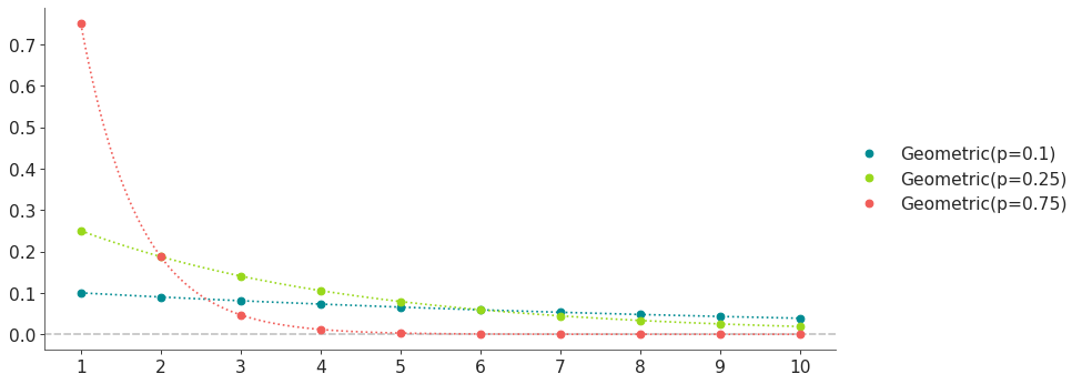

Support	$x \in \mathbb{N}_{>0}$
Mean	$\dfrac{1}{p}$
Variance	$\dfrac{1 - p}{p^2}$

Parameters:: p (float) – Probability of success on an individual trial (0 < p <= 1).

cdf(x)[source]#

Cumulative distribution function.

Parameters:: x (array_like) – Values on which to evaluate the cdf

entropy()[source]#: Entropy.

eti(mass=None, fmt='.2f')#

Equal-tailed interval containing mass.

Parameters:

mass (float) – Probability mass in the interval. Defaults to None,
used. (which results in the value of rcParams["stats.ci_prob"] being)
fmt (str) – fmt used to represent results using f-string fmt for floats. Default to “.2f” i.e. 2 digits after the decimal point. Use “none” for no format.

hdi(mass=None, fmt='.2f')#

Highest density interval containing mass.

Parameters:

mass (float) – Probability mass in the interval. Defaults to None,
used. (which results in the value of rcParams["stats.ci_prob"] being)
fmt (str) – fmt used to represent results using f-string fmt for floats. Default to “.2f” i.e. 2 digits after the decimal point. Use “none” for no format.

isf(x)#

Inverse survival function (inverse of sf).

Parameters:: x (array_like) – Values on which to evaluate the inverse of the sf

kurtosis()[source]#: Excess kurtosis.

lmoment1()[source]#: L-moment1 (mean).

lmoment2()[source]#: L-moment2 (l-scale).

lmoment3()[source]#: L-moment3 (l-skewness). This the ratio of L-moment3 to L-moment2.

lmoment4()[source]#: L-moment4 (l-kurtosis). This the ratio of L-moment4 to L-moment2.

lmoments(types='1234')#

Compute L-moments of the distribution.

Parameters:: types (str) – The type of moments to compute. Default is ‘1234’ where ‘1’ = L-moment1 (mean), ‘2’ = L-moment2 (l-scale), ‘3’ = L-moment3 (l-skewness), and ‘4’ = L-moment4 (l-kurtosis). To compute the standard deviation use ‘d’ Valid combinations are any subset of ‘1234’.

logcdf(x)#

Log cumulative distribution function.

Parameters:: x (array_like) – Values on which to evaluate the logcdf

logpdf(x)[source]#

Log probability density/mass function.

Parameters:: x (array_like) – Values on which to evaluate the logpdf

logsf(x)#

Log survival function log(1 - cdf).

Parameters:: x (array_like) – Values on which to evaluate the logsf

mean()[source]#: Mean.

median()[source]#: Median.

mode()[source]#: Mode.

moments(types='mvsk')#

Compute moments of the distribution.

It can also return the standard deviation

Parameters:: types (str) – The type of moments to compute. Default is ‘mvsk’ where ‘m’ = mean, ‘v’ = variance, ‘s’ = skewness, and ‘k’ = kurtosis. To compute the standard deviation use ‘d’ Valid combinations are any subset of ‘mvdsk’.

pdf(x)[source]#

Probability density/mass function.

Parameters:: x (array_like) – Values on which to evaluate the pdf

plot_cdf(moments=None, pointinterval=False, interval=None, levels=None, support='restricted', legend='legend', figsize=None, ax=None, **kwargs)#

Plot the cumulative distribution function.

Parameters:

moments (str) – Compute moments. Use any combination of the strings m, d, v, s or k for the mean (μ), standard deviation (σ), variance (σ²), skew (γ) or kurtosis (κ) respectively. Other strings will be ignored. Defaults to None.
pointinterval (bool) – Whether to include a plot of the quantiles. Defaults to False. If True the default is to plot the median and two interquantiles ranges.
interval (str) – Type of interval. Available options are highest density interval “hdi” (default), equal tailed interval “eti” or intervals defined by arbitrary “quantiles”. Defaults to the value in rcParams[“stats.ci_kind”].
levels (list) – Mass of the intervals. For hdi or eti the number of elements should be 2 or 1. For quantiles the number of elements should be 5, 3, 1 or 0 (in this last case nothing will be plotted).
support (str:) – If full use the finite end-points to set the limits of the plot. For unbounded end-points or if restricted use the 0.001 and 0.999 quantiles to set the limits.
legend (str) – Whether to include a string with the distribution and its parameter as a "legend" a "title" or not include them None.
figsize (tuple) – Size of the figure
ax (matplotlib axes)
kwargs (keyword arguments) – Additional keyword arguments passed to matplotlib plot function. For example, color, alpha, linewidth, etc.

plot_interactive(kind='pdf', xy_lim='both', pointinterval=True, interval=None, levels=None, figsize=None)#

Interactive exploration of distributions parameters.

Parameters:

kind (str:) – Type of plot. Available options are pdf, cdf and ppf.
xy_lim (str or tuple) – Set the limits of the x-axis and/or y-axis. Defaults to “both”, the limits of both axis are fixed. Use “auto” for automatic rescaling of x-axis and y-axis. Or set them manually by passing a tuple of 4 elements, the first two for x-axis, the last two for y-axis. The tuple can have None.
pointinterval (bool) – Whether to include a plot of the quantiles. Defaults to False. If True the default is to plot the median and two interquantiles ranges.
interval (str) – Type of interval. Available options are highest density interval “hdi” (default), equal tailed interval “eti” or intervals defined by arbitrary “quantiles”. Defaults to the value in rcParams[“stats.ci_kind”].
levels (list) – Mass of the intervals. For hdi or eti the number of elements should be 2 or 1. For quantiles the number of elements should be 5, 3, 1 or 0 (in this last case nothing will be plotted).
figsize (tuple) – Size of the figure

plot_isf(moments=None, pointinterval=False, interval=None, levels=None, legend='legend', figsize=None, ax=None, **kwargs)#

Plot the inverse survival function.

Parameters:

moments (str) – Compute moments. Use any combination of the strings m, d, v, s or k for the mean (μ), standard deviation (σ), variance (σ²), skew (γ) or kurtosis (κ) respectively. Other strings will be ignored. Defaults to None.
pointinterval (bool) – Whether to include a plot of the quantiles. Defaults to False. If True the default is to plot the median and two interquantiles ranges.
interval (str) – Type of interval. Available options are highest density interval “hdi” (default), equal tailed interval “eti” or intervals defined by arbitrary “quantiles”. Defaults to the value in rcParams[“stats.ci_kind”].
levels (list) – Mass of the intervals. For hdi or eti the number of elements should be 2 or 1. For quantiles the number of elements should be 5, 3, 1 or 0 (in this last case nothing will be plotted).
legend (str) – Whether to include a string with the distribution and its parameter as a "legend" a "title" or not include them None.
figsize (tuple) – Size of the figure
ax (matplotlib axes)

plot_pdf(moments=None, pointinterval=False, interval=None, levels=None, support='restricted', baseline=True, legend='legend', figsize=None, ax=None, **kwargs)#

Plot the pdf (continuous) or pmf (discrete).

Parameters:

moments (str) – Compute moments. Use any combination of the strings m, d, v, s or k for the mean (μ), standard deviation (σ), variance (σ²), skew (γ) or kurtosis (κ) respectively. Other strings will be ignored. Defaults to None.
pointinterval (bool) – Whether to include a plot of the quantiles. Defaults to False. If True the default is to plot the median and two interquantiles ranges.
interval (str) – Type of interval. Available options are highest density interval “hdi” (default), equal tailed interval “eti” or intervals defined by arbitrary “quantiles”. Defaults to the value in rcParams[“stats.ci_kind”].
levels (list) – Mass of the intervals. For hdi or eti the number of elements should be 2 or 1. For quantiles the number of elements should be 5, 3, 1 or 0 (in this last case nothing will be plotted).
support (str:) – If full use the finite end-points to set the limits of the plot. For unbounded end-points or if restricted use the 0.001 and 0.999 quantiles to set the limits.
baseline (bool) – Whether to include a horizontal line at y=0.
legend (str) – Whether to include a string with the distribution and its parameter as a "legend" a "title" or not include them None.
figsize (tuple) – Size of the figure
ax (matplotlib axes)
kwargs (keyword arguments) – Additional keyword arguments passed to matplotlib plot function. For example, color, alpha, linewidth, etc.

plot_ppf(moments=None, pointinterval=False, interval=None, levels=None, legend='legend', figsize=None, ax=None, **kwargs)#

Plot the quantile function.

Parameters:

moments (str) – Compute moments. Use any combination of the strings m, d, v, s or k for the mean (μ), standard deviation (σ), variance (σ²), skew (γ) or kurtosis (κ) respectively. Other strings will be ignored. Defaults to None.
pointinterval (bool) – Whether to include a plot of the quantiles. Defaults to False. If True the default is to plot the median and two interquantiles ranges.
interval (str) – Type of interval. Available options are highest density interval “hdi” (default), equal tailed interval “eti” or intervals defined by arbitrary “quantiles”. Defaults to the value in rcParams[“stats.ci_kind”].
levels (list) – Mass of the intervals. For hdi or eti the number of elements should be 2 or 1. For quantiles the number of elements should be 5, 3, 1 or 0 (in this last case nothing will be plotted).
legend (str) – Whether to include a string with the distribution and its parameter as a "legend" a "title" or not include them None.
figsize (tuple) – Size of the figure
ax (matplotlib axes)

plot_sf(moments=None, pointinterval=False, interval=None, levels=None, support='restricted', legend='legend', figsize=None, ax=None, **kwargs)#

Plot the survival distribution function (1 - CDF).

Parameters:

moments (str) – Compute moments. Use any combination of the strings m, d, v, s or k for the mean (μ), standard deviation (σ), variance (σ²), skew (γ) or kurtosis (κ) respectively. Other strings will be ignored. Defaults to None.
pointinterval (bool) – Whether to include a plot of the quantiles. Defaults to False. If True the default is to plot the median and two interquantiles ranges.
interval (str) – Type of interval. Available options are highest density interval “hdi” (default), equal tailed interval “eti” or intervals defined by arbitrary “quantiles”. Defaults to the value in rcParams[“stats.ci_kind”].
levels (list) – Mass of the intervals. For hdi or eti the number of elements should be 2 or 1. For quantiles the number of elements should be 5, 3, 1 or 0 (in this last case nothing will be plotted).
support (str:) – If full use the finite end-points to set the limits of the plot. For unbounded end-points or if restricted use the 0.001 and 0.999 quantiles to set the limits.
legend (str) – Whether to include a string with the distribution and its parameter as a "legend" a "title" or not include them None.
figsize (tuple) – Size of the figure
ax (matplotlib axes)
kwargs (keyword arguments) – Additional keyword arguments passed to matplotlib plot function. For example, color, alpha, linewidth, etc.

ppf(q)[source]#

Percent point function (inverse of cdf).

Parameters:: x (array_like) – Values on which to evaluate the inverse of the cdf

rvs(size=None, random_state=None)[source]#

Random sample.

Parameters:

size (int or tuple of ints, optional) – Defining number of random variates. Defaults to 1.
random_state ({None, int, numpy.random.Generator, numpy.random.RandomState}) – Defaults to None

sf(x)#

Survival function (1 - cdf).

Parameters:: x (array_like) – Values on which to evaluate the sf

skewness()[source]#: Skewness.

std()[source]#: Standard deviation.

summary(mass=None, interval=None, fmt='.2f')#

Namedtuple with the mean, median, sd, and lower and upper bounds.

Parameters:

mass (float) – Probability mass for the equal-tailed interval. Defaults to None,
used. (which results in the value of rcParams["stats.ci_prob"] being)
interval (str or list-like) – Type of interval. Available options are highest density interval “hdi”, equal tailed interval “eti” or arbitrary interval defined by a list-like object with a pair of values. Defaults to the value in rcParams[“stats.ci_kind”].
fmt (str) – fmt used to represent results using f-string fmt for floats. Default to “.2f” i.e. 2 digits after the decimal point.

to_bambi(**kwargs)#

Convert the PreliZ distribution to a Bambi Prior.

kwargsPyMC distributions properties: kwargs are used to specify properties such as shape or dims

Return type:: Bambi Prior

to_pymc(name=None, **kwargs)#

Convert the PreliZ distribution to a PyMC distribution.

namestr: Name of PyMC distribution. Needed if inside Model context
kwargsPyMC distributions properties: kwargs are used to specify properties such as shape or dims

Return type:: PyMC distribution

var()[source]#: Variance.

xvals(support, n_points=None)#

Provide x values in the support of the distribution.

This is useful for example when plotting.

Parameters:

support (str) – Available options are “full” or “restricted”. If “full” the values will cover the entire support of the distribution if the boundary is finite, or the quantiles 0.0001 or 0.9999, if infinite. If “restricted” the values will cover the quantile 0.0001 to 0.9999.
n_points (int) – Number of values to return. Defaults to 1000 for continuous distributions and 200 for discrete ones. For discrete distributions the returned values may be fewer than n_points if the actual number of discrete values in the support of the distribution is smaller than n_points.

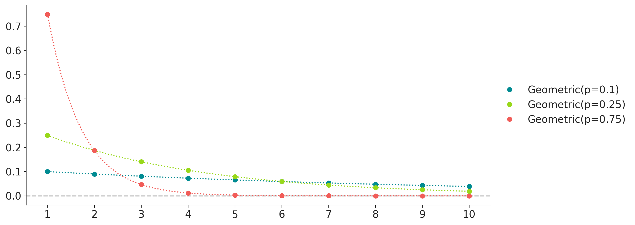
class preliz.distributions.hypergeometric.HyperGeometric(N=None, k=None, n=None)[source]#

Discrete hypergeometric distribution.

The probability of $x$ successes in a sequence of $n$ bernoulli trials taken without replacement from a population of $N$ objects, containing $k$ good (or successful or Type I) objects. The pmf of this distribution is

\[f(x \mid N, n, k) = \frac{\binom{k}{x}\binom{N-k}{n-x}}{\binom{N}{n}}\]

(Source code, png, hires.png, pdf)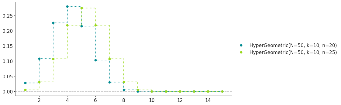

Support	$x \in \left[\max(0, n - N + k), \min(k, n)\right]$
Mean	$\dfrac{nk}{N}$
Variance	$\dfrac{(N-n)nk(N-k)}{(N-1)N^2}$

Parameters:

N (int) – Total size of the population (N > 0)
k (int) – Number of successful individuals in the population (0 <= k <= N)
n (int) – Number of samples drawn from the population (0 <= n <= N)

cdf(x)[source]#

Cumulative distribution function.

Parameters:: x (array_like) – Values on which to evaluate the cdf

entropy()[source]#: Entropy.

eti(mass=None, fmt='.2f')#

Equal-tailed interval containing mass.

Parameters:

mass (float) – Probability mass in the interval. Defaults to None,
used. (which results in the value of rcParams["stats.ci_prob"] being)
fmt (str) – fmt used to represent results using f-string fmt for floats. Default to “.2f” i.e. 2 digits after the decimal point. Use “none” for no format.

hdi(mass=None, fmt='.2f')#

Highest density interval containing mass.

Parameters:

mass (float) – Probability mass in the interval. Defaults to None,
used. (which results in the value of rcParams["stats.ci_prob"] being)
fmt (str) – fmt used to represent results using f-string fmt for floats. Default to “.2f” i.e. 2 digits after the decimal point. Use “none” for no format.

isf(x)#

Inverse survival function (inverse of sf).

Parameters:: x (array_like) – Values on which to evaluate the inverse of the sf

kurtosis()[source]#: Excess kurtosis.

lmoment1()[source]#: L-moment1 (mean).

lmoment2()[source]#: L-moment2 (l-scale).

lmoment3()[source]#: L-moment3 (l-skewness). This the ratio of L-moment3 to L-moment2.

lmoment4()[source]#: L-moment4 (l-kurtosis). This the ratio of L-moment4 to L-moment2.

lmoments(types='1234')#

Compute L-moments of the distribution.

Parameters:: types (str) – The type of moments to compute. Default is ‘1234’ where ‘1’ = L-moment1 (mean), ‘2’ = L-moment2 (l-scale), ‘3’ = L-moment3 (l-skewness), and ‘4’ = L-moment4 (l-kurtosis). To compute the standard deviation use ‘d’ Valid combinations are any subset of ‘1234’.

logcdf(x)#

Log cumulative distribution function.

Parameters:: x (array_like) – Values on which to evaluate the logcdf

logpdf(x)[source]#

Log probability density/mass function.

Parameters:: x (array_like) – Values on which to evaluate the logpdf

logsf(x)#

Log survival function log(1 - cdf).

Parameters:: x (array_like) – Values on which to evaluate the logsf

mean()[source]#: Mean.

median()[source]#: Median.

mode()[source]#: Mode.

moments(types='mvsk')#

Compute moments of the distribution.

It can also return the standard deviation

Parameters:: types (str) – The type of moments to compute. Default is ‘mvsk’ where ‘m’ = mean, ‘v’ = variance, ‘s’ = skewness, and ‘k’ = kurtosis. To compute the standard deviation use ‘d’ Valid combinations are any subset of ‘mvdsk’.

pdf(x)[source]#

Probability density/mass function.

Parameters:: x (array_like) – Values on which to evaluate the pdf

plot_cdf(moments=None, pointinterval=False, interval=None, levels=None, support='restricted', legend='legend', figsize=None, ax=None, **kwargs)#

Plot the cumulative distribution function.

Parameters:

moments (str) – Compute moments. Use any combination of the strings m, d, v, s or k for the mean (μ), standard deviation (σ), variance (σ²), skew (γ) or kurtosis (κ) respectively. Other strings will be ignored. Defaults to None.
pointinterval (bool) – Whether to include a plot of the quantiles. Defaults to False. If True the default is to plot the median and two interquantiles ranges.
interval (str) – Type of interval. Available options are highest density interval “hdi” (default), equal tailed interval “eti” or intervals defined by arbitrary “quantiles”. Defaults to the value in rcParams[“stats.ci_kind”].
levels (list) – Mass of the intervals. For hdi or eti the number of elements should be 2 or 1. For quantiles the number of elements should be 5, 3, 1 or 0 (in this last case nothing will be plotted).
support (str:) – If full use the finite end-points to set the limits of the plot. For unbounded end-points or if restricted use the 0.001 and 0.999 quantiles to set the limits.
legend (str) – Whether to include a string with the distribution and its parameter as a "legend" a "title" or not include them None.
figsize (tuple) – Size of the figure
ax (matplotlib axes)
kwargs (keyword arguments) – Additional keyword arguments passed to matplotlib plot function. For example, color, alpha, linewidth, etc.

plot_interactive(kind='pdf', xy_lim='both', pointinterval=True, interval=None, levels=None, figsize=None)#

Interactive exploration of distributions parameters.

Parameters:

kind (str:) – Type of plot. Available options are pdf, cdf and ppf.
xy_lim (str or tuple) – Set the limits of the x-axis and/or y-axis. Defaults to “both”, the limits of both axis are fixed. Use “auto” for automatic rescaling of x-axis and y-axis. Or set them manually by passing a tuple of 4 elements, the first two for x-axis, the last two for y-axis. The tuple can have None.
pointinterval (bool) – Whether to include a plot of the quantiles. Defaults to False. If True the default is to plot the median and two interquantiles ranges.
interval (str) – Type of interval. Available options are highest density interval “hdi” (default), equal tailed interval “eti” or intervals defined by arbitrary “quantiles”. Defaults to the value in rcParams[“stats.ci_kind”].
levels (list) – Mass of the intervals. For hdi or eti the number of elements should be 2 or 1. For quantiles the number of elements should be 5, 3, 1 or 0 (in this last case nothing will be plotted).
figsize (tuple) – Size of the figure

plot_isf(moments=None, pointinterval=False, interval=None, levels=None, legend='legend', figsize=None, ax=None, **kwargs)#

Plot the inverse survival function.

Parameters:

moments (str) – Compute moments. Use any combination of the strings m, d, v, s or k for the mean (μ), standard deviation (σ), variance (σ²), skew (γ) or kurtosis (κ) respectively. Other strings will be ignored. Defaults to None.
pointinterval (bool) – Whether to include a plot of the quantiles. Defaults to False. If True the default is to plot the median and two interquantiles ranges.
interval (str) – Type of interval. Available options are highest density interval “hdi” (default), equal tailed interval “eti” or intervals defined by arbitrary “quantiles”. Defaults to the value in rcParams[“stats.ci_kind”].
levels (list) – Mass of the intervals. For hdi or eti the number of elements should be 2 or 1. For quantiles the number of elements should be 5, 3, 1 or 0 (in this last case nothing will be plotted).
legend (str) – Whether to include a string with the distribution and its parameter as a "legend" a "title" or not include them None.
figsize (tuple) – Size of the figure
ax (matplotlib axes)

plot_pdf(moments=None, pointinterval=False, interval=None, levels=None, support='restricted', baseline=True, legend='legend', figsize=None, ax=None, **kwargs)#

Plot the pdf (continuous) or pmf (discrete).

Parameters:

moments (str) – Compute moments. Use any combination of the strings m, d, v, s or k for the mean (μ), standard deviation (σ), variance (σ²), skew (γ) or kurtosis (κ) respectively. Other strings will be ignored. Defaults to None.
pointinterval (bool) – Whether to include a plot of the quantiles. Defaults to False. If True the default is to plot the median and two interquantiles ranges.
interval (str) – Type of interval. Available options are highest density interval “hdi” (default), equal tailed interval “eti” or intervals defined by arbitrary “quantiles”. Defaults to the value in rcParams[“stats.ci_kind”].
levels (list) – Mass of the intervals. For hdi or eti the number of elements should be 2 or 1. For quantiles the number of elements should be 5, 3, 1 or 0 (in this last case nothing will be plotted).
support (str:) – If full use the finite end-points to set the limits of the plot. For unbounded end-points or if restricted use the 0.001 and 0.999 quantiles to set the limits.
baseline (bool) – Whether to include a horizontal line at y=0.
legend (str) – Whether to include a string with the distribution and its parameter as a "legend" a "title" or not include them None.
figsize (tuple) – Size of the figure
ax (matplotlib axes)
kwargs (keyword arguments) – Additional keyword arguments passed to matplotlib plot function. For example, color, alpha, linewidth, etc.

plot_ppf(moments=None, pointinterval=False, interval=None, levels=None, legend='legend', figsize=None, ax=None, **kwargs)#

Plot the quantile function.

Parameters:

moments (str) – Compute moments. Use any combination of the strings m, d, v, s or k for the mean (μ), standard deviation (σ), variance (σ²), skew (γ) or kurtosis (κ) respectively. Other strings will be ignored. Defaults to None.
pointinterval (bool) – Whether to include a plot of the quantiles. Defaults to False. If True the default is to plot the median and two interquantiles ranges.
interval (str) – Type of interval. Available options are highest density interval “hdi” (default), equal tailed interval “eti” or intervals defined by arbitrary “quantiles”. Defaults to the value in rcParams[“stats.ci_kind”].
levels (list) – Mass of the intervals. For hdi or eti the number of elements should be 2 or 1. For quantiles the number of elements should be 5, 3, 1 or 0 (in this last case nothing will be plotted).
legend (str) – Whether to include a string with the distribution and its parameter as a "legend" a "title" or not include them None.
figsize (tuple) – Size of the figure
ax (matplotlib axes)

plot_sf(moments=None, pointinterval=False, interval=None, levels=None, support='restricted', legend='legend', figsize=None, ax=None, **kwargs)#

Plot the survival distribution function (1 - CDF).

Parameters:

moments (str) – Compute moments. Use any combination of the strings m, d, v, s or k for the mean (μ), standard deviation (σ), variance (σ²), skew (γ) or kurtosis (κ) respectively. Other strings will be ignored. Defaults to None.
pointinterval (bool) – Whether to include a plot of the quantiles. Defaults to False. If True the default is to plot the median and two interquantiles ranges.
interval (str) – Type of interval. Available options are highest density interval “hdi” (default), equal tailed interval “eti” or intervals defined by arbitrary “quantiles”. Defaults to the value in rcParams[“stats.ci_kind”].
levels (list) – Mass of the intervals. For hdi or eti the number of elements should be 2 or 1. For quantiles the number of elements should be 5, 3, 1 or 0 (in this last case nothing will be plotted).
support (str:) – If full use the finite end-points to set the limits of the plot. For unbounded end-points or if restricted use the 0.001 and 0.999 quantiles to set the limits.
legend (str) – Whether to include a string with the distribution and its parameter as a "legend" a "title" or not include them None.
figsize (tuple) – Size of the figure
ax (matplotlib axes)
kwargs (keyword arguments) – Additional keyword arguments passed to matplotlib plot function. For example, color, alpha, linewidth, etc.

ppf(q)[source]#

Percent point function (inverse of cdf).

Parameters:: x (array_like) – Values on which to evaluate the inverse of the cdf

rvs(size=None, random_state=None)[source]#

Random sample.

Parameters:

size (int or tuple of ints, optional) – Defining number of random variates. Defaults to 1.
random_state ({None, int, numpy.random.Generator, numpy.random.RandomState}) – Defaults to None

sf(x)#

Survival function (1 - cdf).

Parameters:: x (array_like) – Values on which to evaluate the sf

skewness()[source]#: Skewness.

std()[source]#: Standard deviation.

summary(mass=None, interval=None, fmt='.2f')#

Namedtuple with the mean, median, sd, and lower and upper bounds.

Parameters:

mass (float) – Probability mass for the equal-tailed interval. Defaults to None,
used. (which results in the value of rcParams["stats.ci_prob"] being)
interval (str or list-like) – Type of interval. Available options are highest density interval “hdi”, equal tailed interval “eti” or arbitrary interval defined by a list-like object with a pair of values. Defaults to the value in rcParams[“stats.ci_kind”].
fmt (str) – fmt used to represent results using f-string fmt for floats. Default to “.2f” i.e. 2 digits after the decimal point.

to_bambi(**kwargs)#

Convert the PreliZ distribution to a Bambi Prior.

kwargsPyMC distributions properties: kwargs are used to specify properties such as shape or dims

Return type:: Bambi Prior

to_pymc(name=None, **kwargs)#

Convert the PreliZ distribution to a PyMC distribution.

namestr: Name of PyMC distribution. Needed if inside Model context
kwargsPyMC distributions properties: kwargs are used to specify properties such as shape or dims

Return type:: PyMC distribution

var()[source]#: Variance.

xvals(support, n_points=None)#

Provide x values in the support of the distribution.

This is useful for example when plotting.

Parameters:

support (str) – Available options are “full” or “restricted”. If “full” the values will cover the entire support of the distribution if the boundary is finite, or the quantiles 0.0001 or 0.9999, if infinite. If “restricted” the values will cover the quantile 0.0001 to 0.9999.
n_points (int) – Number of values to return. Defaults to 1000 for continuous distributions and 200 for discrete ones. For discrete distributions the returned values may be fewer than n_points if the actual number of discrete values in the support of the distribution is smaller than n_points.

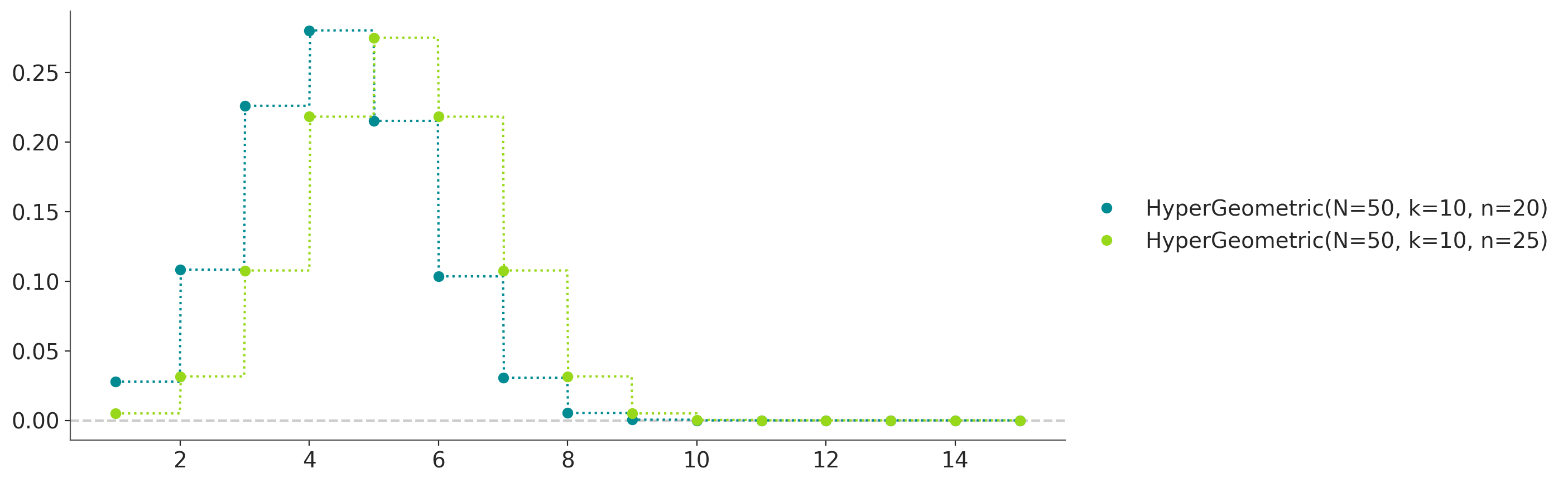
class preliz.distributions.poisson.Poisson(mu=None)[source]#

Poisson distribution.

Often used to model the number of events occurring in a fixed period of time when the times at which events occur are independent. The pmf of this distribution is

\[f(x \mid \mu) = \frac{e^{-\mu}\mu^x}{x!}\]

(Source code, png, hires.png, pdf)

Support	$x \in \mathbb{N}_0$
Mean	$\mu$
Variance	$\mu$

Parameters:: mu (float) – Expected number of occurrences during the given interval (mu >= 0).

Notes

The Poisson distribution can be derived as a limiting case of the binomial distribution.

cdf(x)[source]#

Cumulative distribution function.

Parameters:: x (array_like) – Values on which to evaluate the cdf

entropy()[source]#: Entropy.

eti(mass=None, fmt='.2f')#

Equal-tailed interval containing mass.

Parameters:

mass (float) – Probability mass in the interval. Defaults to None,
used. (which results in the value of rcParams["stats.ci_prob"] being)
fmt (str) – fmt used to represent results using f-string fmt for floats. Default to “.2f” i.e. 2 digits after the decimal point. Use “none” for no format.

hdi(mass=None, fmt='.2f')#

Highest density interval containing mass.

Parameters:

mass (float) – Probability mass in the interval. Defaults to None,
used. (which results in the value of rcParams["stats.ci_prob"] being)
fmt (str) – fmt used to represent results using f-string fmt for floats. Default to “.2f” i.e. 2 digits after the decimal point. Use “none” for no format.

isf(x)#

Inverse survival function (inverse of sf).

Parameters:: x (array_like) – Values on which to evaluate the inverse of the sf

kurtosis()[source]#: Excess kurtosis.

lmoment1()[source]#: L-moment1 (mean).

lmoment2()[source]#: L-moment2 (l-scale).

lmoment3()[source]#: L-moment3 (l-skewness). This the ratio of L-moment3 to L-moment2.

lmoment4()[source]#: L-moment4 (l-kurtosis). This the ratio of L-moment4 to L-moment2.

lmoments(types='1234')#

Compute L-moments of the distribution.

Parameters:: types (str) – The type of moments to compute. Default is ‘1234’ where ‘1’ = L-moment1 (mean), ‘2’ = L-moment2 (l-scale), ‘3’ = L-moment3 (l-skewness), and ‘4’ = L-moment4 (l-kurtosis). To compute the standard deviation use ‘d’ Valid combinations are any subset of ‘1234’.

logcdf(x)#

Log cumulative distribution function.

Parameters:: x (array_like) – Values on which to evaluate the logcdf

logpdf(x)[source]#

Log probability density/mass function.

Parameters:: x (array_like) – Values on which to evaluate the logpdf

logsf(x)#

Log survival function log(1 - cdf).

Parameters:: x (array_like) – Values on which to evaluate the logsf

mean()[source]#: Mean.

median()[source]#: Median.

mode()[source]#: Mode.

moments(types='mvsk')#

Compute moments of the distribution.

It can also return the standard deviation

Parameters:: types (str) – The type of moments to compute. Default is ‘mvsk’ where ‘m’ = mean, ‘v’ = variance, ‘s’ = skewness, and ‘k’ = kurtosis. To compute the standard deviation use ‘d’ Valid combinations are any subset of ‘mvdsk’.

pdf(x)[source]#

Probability density/mass function.

Parameters:: x (array_like) – Values on which to evaluate the pdf

plot_cdf(moments=None, pointinterval=False, interval=None, levels=None, support='restricted', legend='legend', figsize=None, ax=None, **kwargs)#

Plot the cumulative distribution function.

Parameters:

moments (str) – Compute moments. Use any combination of the strings m, d, v, s or k for the mean (μ), standard deviation (σ), variance (σ²), skew (γ) or kurtosis (κ) respectively. Other strings will be ignored. Defaults to None.
pointinterval (bool) – Whether to include a plot of the quantiles. Defaults to False. If True the default is to plot the median and two interquantiles ranges.
interval (str) – Type of interval. Available options are highest density interval “hdi” (default), equal tailed interval “eti” or intervals defined by arbitrary “quantiles”. Defaults to the value in rcParams[“stats.ci_kind”].
levels (list) – Mass of the intervals. For hdi or eti the number of elements should be 2 or 1. For quantiles the number of elements should be 5, 3, 1 or 0 (in this last case nothing will be plotted).
support (str:) – If full use the finite end-points to set the limits of the plot. For unbounded end-points or if restricted use the 0.001 and 0.999 quantiles to set the limits.
legend (str) – Whether to include a string with the distribution and its parameter as a "legend" a "title" or not include them None.
figsize (tuple) – Size of the figure
ax (matplotlib axes)
kwargs (keyword arguments) – Additional keyword arguments passed to matplotlib plot function. For example, color, alpha, linewidth, etc.

plot_interactive(kind='pdf', xy_lim='both', pointinterval=True, interval=None, levels=None, figsize=None)#

Interactive exploration of distributions parameters.

Parameters:

kind (str:) – Type of plot. Available options are pdf, cdf and ppf.
xy_lim (str or tuple) – Set the limits of the x-axis and/or y-axis. Defaults to “both”, the limits of both axis are fixed. Use “auto” for automatic rescaling of x-axis and y-axis. Or set them manually by passing a tuple of 4 elements, the first two for x-axis, the last two for y-axis. The tuple can have None.
pointinterval (bool) – Whether to include a plot of the quantiles. Defaults to False. If True the default is to plot the median and two interquantiles ranges.
interval (str) – Type of interval. Available options are highest density interval “hdi” (default), equal tailed interval “eti” or intervals defined by arbitrary “quantiles”. Defaults to the value in rcParams[“stats.ci_kind”].
levels (list) – Mass of the intervals. For hdi or eti the number of elements should be 2 or 1. For quantiles the number of elements should be 5, 3, 1 or 0 (in this last case nothing will be plotted).
figsize (tuple) – Size of the figure

plot_isf(moments=None, pointinterval=False, interval=None, levels=None, legend='legend', figsize=None, ax=None, **kwargs)#

Plot the inverse survival function.

Parameters:

moments (str) – Compute moments. Use any combination of the strings m, d, v, s or k for the mean (μ), standard deviation (σ), variance (σ²), skew (γ) or kurtosis (κ) respectively. Other strings will be ignored. Defaults to None.
pointinterval (bool) – Whether to include a plot of the quantiles. Defaults to False. If True the default is to plot the median and two interquantiles ranges.
interval (str) – Type of interval. Available options are highest density interval “hdi” (default), equal tailed interval “eti” or intervals defined by arbitrary “quantiles”. Defaults to the value in rcParams[“stats.ci_kind”].
levels (list) – Mass of the intervals. For hdi or eti the number of elements should be 2 or 1. For quantiles the number of elements should be 5, 3, 1 or 0 (in this last case nothing will be plotted).
legend (str) – Whether to include a string with the distribution and its parameter as a "legend" a "title" or not include them None.
figsize (tuple) – Size of the figure
ax (matplotlib axes)

plot_pdf(moments=None, pointinterval=False, interval=None, levels=None, support='restricted', baseline=True, legend='legend', figsize=None, ax=None, **kwargs)#

Plot the pdf (continuous) or pmf (discrete).

Parameters:

moments (str) – Compute moments. Use any combination of the strings m, d, v, s or k for the mean (μ), standard deviation (σ), variance (σ²), skew (γ) or kurtosis (κ) respectively. Other strings will be ignored. Defaults to None.
pointinterval (bool) – Whether to include a plot of the quantiles. Defaults to False. If True the default is to plot the median and two interquantiles ranges.
interval (str) – Type of interval. Available options are highest density interval “hdi” (default), equal tailed interval “eti” or intervals defined by arbitrary “quantiles”. Defaults to the value in rcParams[“stats.ci_kind”].
levels (list) – Mass of the intervals. For hdi or eti the number of elements should be 2 or 1. For quantiles the number of elements should be 5, 3, 1 or 0 (in this last case nothing will be plotted).
support (str:) – If full use the finite end-points to set the limits of the plot. For unbounded end-points or if restricted use the 0.001 and 0.999 quantiles to set the limits.
baseline (bool) – Whether to include a horizontal line at y=0.
legend (str) – Whether to include a string with the distribution and its parameter as a "legend" a "title" or not include them None.
figsize (tuple) – Size of the figure
ax (matplotlib axes)
kwargs (keyword arguments) – Additional keyword arguments passed to matplotlib plot function. For example, color, alpha, linewidth, etc.

plot_ppf(moments=None, pointinterval=False, interval=None, levels=None, legend='legend', figsize=None, ax=None, **kwargs)#

Plot the quantile function.

Parameters:

moments (str) – Compute moments. Use any combination of the strings m, d, v, s or k for the mean (μ), standard deviation (σ), variance (σ²), skew (γ) or kurtosis (κ) respectively. Other strings will be ignored. Defaults to None.
pointinterval (bool) – Whether to include a plot of the quantiles. Defaults to False. If True the default is to plot the median and two interquantiles ranges.
interval (str) – Type of interval. Available options are highest density interval “hdi” (default), equal tailed interval “eti” or intervals defined by arbitrary “quantiles”. Defaults to the value in rcParams[“stats.ci_kind”].
levels (list) – Mass of the intervals. For hdi or eti the number of elements should be 2 or 1. For quantiles the number of elements should be 5, 3, 1 or 0 (in this last case nothing will be plotted).
legend (str) – Whether to include a string with the distribution and its parameter as a "legend" a "title" or not include them None.
figsize (tuple) – Size of the figure
ax (matplotlib axes)

plot_sf(moments=None, pointinterval=False, interval=None, levels=None, support='restricted', legend='legend', figsize=None, ax=None, **kwargs)#

Plot the survival distribution function (1 - CDF).

Parameters:

moments (str) – Compute moments. Use any combination of the strings m, d, v, s or k for the mean (μ), standard deviation (σ), variance (σ²), skew (γ) or kurtosis (κ) respectively. Other strings will be ignored. Defaults to None.
pointinterval (bool) – Whether to include a plot of the quantiles. Defaults to False. If True the default is to plot the median and two interquantiles ranges.
interval (str) – Type of interval. Available options are highest density interval “hdi” (default), equal tailed interval “eti” or intervals defined by arbitrary “quantiles”. Defaults to the value in rcParams[“stats.ci_kind”].
levels (list) – Mass of the intervals. For hdi or eti the number of elements should be 2 or 1. For quantiles the number of elements should be 5, 3, 1 or 0 (in this last case nothing will be plotted).
support (str:) – If full use the finite end-points to set the limits of the plot. For unbounded end-points or if restricted use the 0.001 and 0.999 quantiles to set the limits.
legend (str) – Whether to include a string with the distribution and its parameter as a "legend" a "title" or not include them None.
figsize (tuple) – Size of the figure
ax (matplotlib axes)
kwargs (keyword arguments) – Additional keyword arguments passed to matplotlib plot function. For example, color, alpha, linewidth, etc.

ppf(q)[source]#

Percent point function (inverse of cdf).

Parameters:: x (array_like) – Values on which to evaluate the inverse of the cdf

rvs(size=None, random_state=None)[source]#

Random sample.

Parameters:

size (int or tuple of ints, optional) – Defining number of random variates. Defaults to 1.
random_state ({None, int, numpy.random.Generator, numpy.random.RandomState}) – Defaults to None

sf(x)#

Survival function (1 - cdf).

Parameters:: x (array_like) – Values on which to evaluate the sf

skewness()[source]#: Skewness.

std()[source]#: Standard deviation.

summary(mass=None, interval=None, fmt='.2f')#

Namedtuple with the mean, median, sd, and lower and upper bounds.

Parameters:

mass (float) – Probability mass for the equal-tailed interval. Defaults to None,
used. (which results in the value of rcParams["stats.ci_prob"] being)
interval (str or list-like) – Type of interval. Available options are highest density interval “hdi”, equal tailed interval “eti” or arbitrary interval defined by a list-like object with a pair of values. Defaults to the value in rcParams[“stats.ci_kind”].
fmt (str) – fmt used to represent results using f-string fmt for floats. Default to “.2f” i.e. 2 digits after the decimal point.

to_bambi(**kwargs)#

Convert the PreliZ distribution to a Bambi Prior.

kwargsPyMC distributions properties: kwargs are used to specify properties such as shape or dims

Return type:: Bambi Prior

to_pymc(name=None, **kwargs)#

Convert the PreliZ distribution to a PyMC distribution.

namestr: Name of PyMC distribution. Needed if inside Model context
kwargsPyMC distributions properties: kwargs are used to specify properties such as shape or dims

Return type:: PyMC distribution

var()[source]#: Variance.

xvals(support, n_points=None)#

Provide x values in the support of the distribution.

This is useful for example when plotting.

Parameters:

support (str) – Available options are “full” or “restricted”. If “full” the values will cover the entire support of the distribution if the boundary is finite, or the quantiles 0.0001 or 0.9999, if infinite. If “restricted” the values will cover the quantile 0.0001 to 0.9999.
n_points (int) – Number of values to return. Defaults to 1000 for continuous distributions and 200 for discrete ones. For discrete distributions the returned values may be fewer than n_points if the actual number of discrete values in the support of the distribution is smaller than n_points.

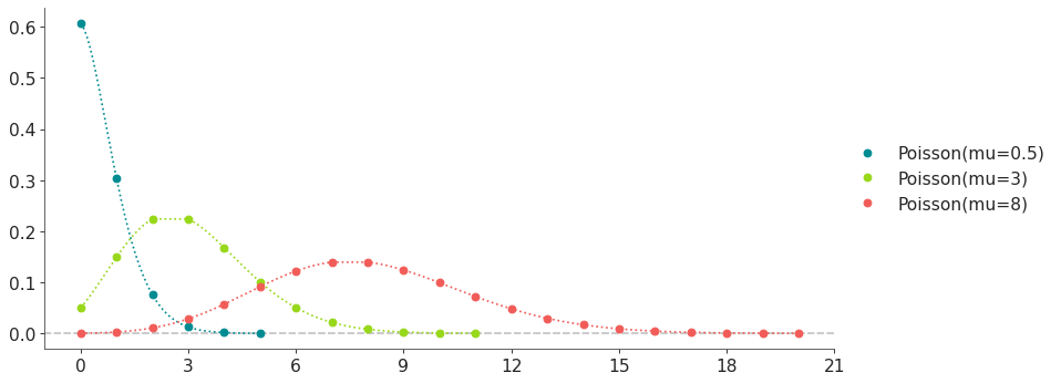
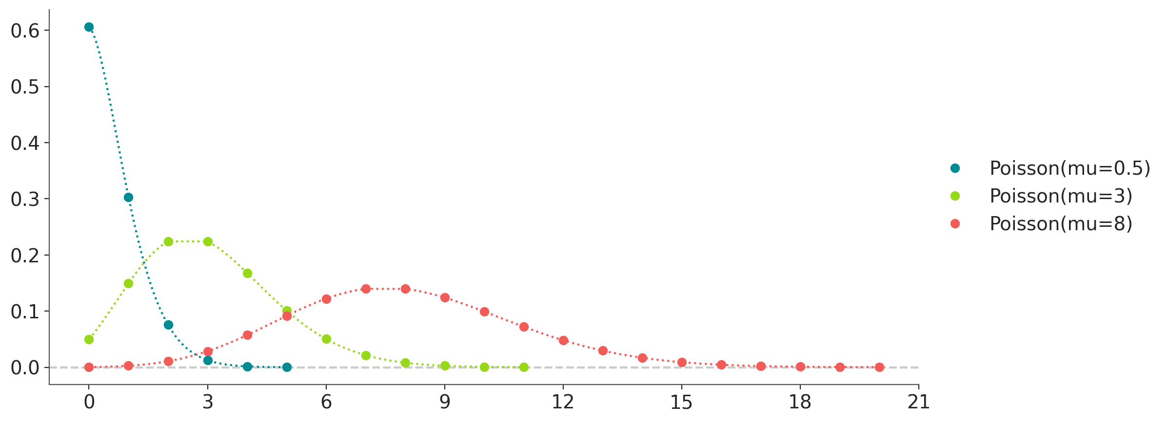
class preliz.distributions.negativebinomial.NegativeBinomial(mu=None, alpha=None, p=None, n=None)[source]#

Negative binomial distribution.

The negative binomial distribution describes a Poisson random variable whose rate parameter is gamma distributed. Its pmf, parametrized by the parameters alpha and mu of the gamma distribution, is

\[f(x \mid \mu, \alpha) = \binom{x + \alpha - 1}{x} (\alpha/(\mu+\alpha))^\alpha (\mu/(\mu+\alpha))^x\]

(Source code, png, hires.png, pdf)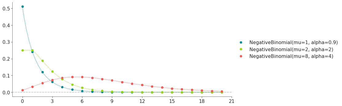

Support	$x \in \mathbb{N}_0$
Mean	$\mu$
Variance	$\frac{\mu (\alpha + \mu)}{\alpha}$

The negative binomial distribution can be parametrized either in terms of mu and alpha, or in terms of n and p. The link between the parametrizations is given by

\[\begin{split}p &= \frac{\alpha}{\mu + \alpha} \\ n &= \alpha\end{split}\]

If it is parametrized in terms of n and p, the negative binomial describes the probability to have x failures before the n-th success, given the probability p of success in each trial. Its pmf is

\[f(x \mid n, p) = \binom{x + n - 1}{x} (p)^n (1 - p)^x\]

Parameters:

alpha (float) – Gamma distribution shape parameter (alpha > 0).
mu (float) – Gamma distribution mean (mu > 0).
p (float) – Probability of success in each trial (0 < p < 1).
n (float) – Number of target success trials (n > 0)

cdf(x)[source]#

Cumulative distribution function.

Parameters:: x (array_like) – Values on which to evaluate the cdf

entropy()[source]#: Entropy.

eti(mass=None, fmt='.2f')#

Equal-tailed interval containing mass.

Parameters:

mass (float) – Probability mass in the interval. Defaults to None,
used. (which results in the value of rcParams["stats.ci_prob"] being)
fmt (str) – fmt used to represent results using f-string fmt for floats. Default to “.2f” i.e. 2 digits after the decimal point. Use “none” for no format.

hdi(mass=None, fmt='.2f')#

Highest density interval containing mass.

Parameters:

mass (float) – Probability mass in the interval. Defaults to None,
used. (which results in the value of rcParams["stats.ci_prob"] being)
fmt (str) – fmt used to represent results using f-string fmt for floats. Default to “.2f” i.e. 2 digits after the decimal point. Use “none” for no format.

isf(x)#

Inverse survival function (inverse of sf).

Parameters:: x (array_like) – Values on which to evaluate the inverse of the sf

kurtosis()[source]#: Excess kurtosis.

lmoment1()[source]#: L-moment1 (mean).

lmoment2()[source]#: L-moment2 (l-scale).

lmoment3()[source]#: L-moment3 (l-skewness). This the ratio of L-moment3 to L-moment2.

lmoment4()[source]#: L-moment4 (l-kurtosis). This the ratio of L-moment4 to L-moment2.

lmoments(types='1234')#

Compute L-moments of the distribution.

Parameters:: types (str) – The type of moments to compute. Default is ‘1234’ where ‘1’ = L-moment1 (mean), ‘2’ = L-moment2 (l-scale), ‘3’ = L-moment3 (l-skewness), and ‘4’ = L-moment4 (l-kurtosis). To compute the standard deviation use ‘d’ Valid combinations are any subset of ‘1234’.

logcdf(x)#

Log cumulative distribution function.

Parameters:: x (array_like) – Values on which to evaluate the logcdf

logpdf(x)[source]#

Log probability density/mass function.

Parameters:: x (array_like) – Values on which to evaluate the logpdf

logsf(x)#

Log survival function log(1 - cdf).

Parameters:: x (array_like) – Values on which to evaluate the logsf

mean()[source]#: Mean.

median()[source]#: Median.

mode()[source]#: Mode.

moments(types='mvsk')#

Compute moments of the distribution.

It can also return the standard deviation

Parameters:: types (str) – The type of moments to compute. Default is ‘mvsk’ where ‘m’ = mean, ‘v’ = variance, ‘s’ = skewness, and ‘k’ = kurtosis. To compute the standard deviation use ‘d’ Valid combinations are any subset of ‘mvdsk’.

pdf(x)[source]#

Probability density/mass function.

Parameters:: x (array_like) – Values on which to evaluate the pdf

plot_cdf(moments=None, pointinterval=False, interval=None, levels=None, support='restricted', legend='legend', figsize=None, ax=None, **kwargs)#

Plot the cumulative distribution function.

Parameters:

moments (str) – Compute moments. Use any combination of the strings m, d, v, s or k for the mean (μ), standard deviation (σ), variance (σ²), skew (γ) or kurtosis (κ) respectively. Other strings will be ignored. Defaults to None.
pointinterval (bool) – Whether to include a plot of the quantiles. Defaults to False. If True the default is to plot the median and two interquantiles ranges.
interval (str) – Type of interval. Available options are highest density interval “hdi” (default), equal tailed interval “eti” or intervals defined by arbitrary “quantiles”. Defaults to the value in rcParams[“stats.ci_kind”].
levels (list) – Mass of the intervals. For hdi or eti the number of elements should be 2 or 1. For quantiles the number of elements should be 5, 3, 1 or 0 (in this last case nothing will be plotted).
support (str:) – If full use the finite end-points to set the limits of the plot. For unbounded end-points or if restricted use the 0.001 and 0.999 quantiles to set the limits.
legend (str) – Whether to include a string with the distribution and its parameter as a "legend" a "title" or not include them None.
figsize (tuple) – Size of the figure
ax (matplotlib axes)
kwargs (keyword arguments) – Additional keyword arguments passed to matplotlib plot function. For example, color, alpha, linewidth, etc.

plot_interactive(kind='pdf', xy_lim='both', pointinterval=True, interval=None, levels=None, figsize=None)#

Interactive exploration of distributions parameters.

Parameters:

kind (str:) – Type of plot. Available options are pdf, cdf and ppf.
xy_lim (str or tuple) – Set the limits of the x-axis and/or y-axis. Defaults to “both”, the limits of both axis are fixed. Use “auto” for automatic rescaling of x-axis and y-axis. Or set them manually by passing a tuple of 4 elements, the first two for x-axis, the last two for y-axis. The tuple can have None.
pointinterval (bool) – Whether to include a plot of the quantiles. Defaults to False. If True the default is to plot the median and two interquantiles ranges.
interval (str) – Type of interval. Available options are highest density interval “hdi” (default), equal tailed interval “eti” or intervals defined by arbitrary “quantiles”. Defaults to the value in rcParams[“stats.ci_kind”].
levels (list) – Mass of the intervals. For hdi or eti the number of elements should be 2 or 1. For quantiles the number of elements should be 5, 3, 1 or 0 (in this last case nothing will be plotted).
figsize (tuple) – Size of the figure

plot_isf(moments=None, pointinterval=False, interval=None, levels=None, legend='legend', figsize=None, ax=None, **kwargs)#

Plot the inverse survival function.

Parameters:

moments (str) – Compute moments. Use any combination of the strings m, d, v, s or k for the mean (μ), standard deviation (σ), variance (σ²), skew (γ) or kurtosis (κ) respectively. Other strings will be ignored. Defaults to None.
pointinterval (bool) – Whether to include a plot of the quantiles. Defaults to False. If True the default is to plot the median and two interquantiles ranges.
interval (str) – Type of interval. Available options are highest density interval “hdi” (default), equal tailed interval “eti” or intervals defined by arbitrary “quantiles”. Defaults to the value in rcParams[“stats.ci_kind”].
levels (list) – Mass of the intervals. For hdi or eti the number of elements should be 2 or 1. For quantiles the number of elements should be 5, 3, 1 or 0 (in this last case nothing will be plotted).
legend (str) – Whether to include a string with the distribution and its parameter as a "legend" a "title" or not include them None.
figsize (tuple) – Size of the figure
ax (matplotlib axes)

plot_pdf(moments=None, pointinterval=False, interval=None, levels=None, support='restricted', baseline=True, legend='legend', figsize=None, ax=None, **kwargs)#

Plot the pdf (continuous) or pmf (discrete).

Parameters:

moments (str) – Compute moments. Use any combination of the strings m, d, v, s or k for the mean (μ), standard deviation (σ), variance (σ²), skew (γ) or kurtosis (κ) respectively. Other strings will be ignored. Defaults to None.
pointinterval (bool) – Whether to include a plot of the quantiles. Defaults to False. If True the default is to plot the median and two interquantiles ranges.
interval (str) – Type of interval. Available options are highest density interval “hdi” (default), equal tailed interval “eti” or intervals defined by arbitrary “quantiles”. Defaults to the value in rcParams[“stats.ci_kind”].
levels (list) – Mass of the intervals. For hdi or eti the number of elements should be 2 or 1. For quantiles the number of elements should be 5, 3, 1 or 0 (in this last case nothing will be plotted).
support (str:) – If full use the finite end-points to set the limits of the plot. For unbounded end-points or if restricted use the 0.001 and 0.999 quantiles to set the limits.
baseline (bool) – Whether to include a horizontal line at y=0.
legend (str) – Whether to include a string with the distribution and its parameter as a "legend" a "title" or not include them None.
figsize (tuple) – Size of the figure
ax (matplotlib axes)
kwargs (keyword arguments) – Additional keyword arguments passed to matplotlib plot function. For example, color, alpha, linewidth, etc.

plot_ppf(moments=None, pointinterval=False, interval=None, levels=None, legend='legend', figsize=None, ax=None, **kwargs)#

Plot the quantile function.

Parameters:

moments (str) – Compute moments. Use any combination of the strings m, d, v, s or k for the mean (μ), standard deviation (σ), variance (σ²), skew (γ) or kurtosis (κ) respectively. Other strings will be ignored. Defaults to None.
pointinterval (bool) – Whether to include a plot of the quantiles. Defaults to False. If True the default is to plot the median and two interquantiles ranges.
interval (str) – Type of interval. Available options are highest density interval “hdi” (default), equal tailed interval “eti” or intervals defined by arbitrary “quantiles”. Defaults to the value in rcParams[“stats.ci_kind”].
levels (list) – Mass of the intervals. For hdi or eti the number of elements should be 2 or 1. For quantiles the number of elements should be 5, 3, 1 or 0 (in this last case nothing will be plotted).
legend (str) – Whether to include a string with the distribution and its parameter as a "legend" a "title" or not include them None.
figsize (tuple) – Size of the figure
ax (matplotlib axes)

plot_sf(moments=None, pointinterval=False, interval=None, levels=None, support='restricted', legend='legend', figsize=None, ax=None, **kwargs)#

Plot the survival distribution function (1 - CDF).

Parameters:

moments (str) – Compute moments. Use any combination of the strings m, d, v, s or k for the mean (μ), standard deviation (σ), variance (σ²), skew (γ) or kurtosis (κ) respectively. Other strings will be ignored. Defaults to None.
pointinterval (bool) – Whether to include a plot of the quantiles. Defaults to False. If True the default is to plot the median and two interquantiles ranges.
interval (str) – Type of interval. Available options are highest density interval “hdi” (default), equal tailed interval “eti” or intervals defined by arbitrary “quantiles”. Defaults to the value in rcParams[“stats.ci_kind”].
levels (list) – Mass of the intervals. For hdi or eti the number of elements should be 2 or 1. For quantiles the number of elements should be 5, 3, 1 or 0 (in this last case nothing will be plotted).
support (str:) – If full use the finite end-points to set the limits of the plot. For unbounded end-points or if restricted use the 0.001 and 0.999 quantiles to set the limits.
legend (str) – Whether to include a string with the distribution and its parameter as a "legend" a "title" or not include them None.
figsize (tuple) – Size of the figure
ax (matplotlib axes)
kwargs (keyword arguments) – Additional keyword arguments passed to matplotlib plot function. For example, color, alpha, linewidth, etc.

ppf(q)[source]#

Percent point function (inverse of cdf).

Parameters:: x (array_like) – Values on which to evaluate the inverse of the cdf

rvs(size=None, random_state=None)[source]#

Random sample.

Parameters:

size (int or tuple of ints, optional) – Defining number of random variates. Defaults to 1.
random_state ({None, int, numpy.random.Generator, numpy.random.RandomState}) – Defaults to None

sf(x)#

Survival function (1 - cdf).

Parameters:: x (array_like) – Values on which to evaluate the sf

skewness()[source]#: Skewness.

std()[source]#: Standard deviation.

summary(mass=None, interval=None, fmt='.2f')#

Namedtuple with the mean, median, sd, and lower and upper bounds.

Parameters:

mass (float) – Probability mass for the equal-tailed interval. Defaults to None,
used. (which results in the value of rcParams["stats.ci_prob"] being)
interval (str or list-like) – Type of interval. Available options are highest density interval “hdi”, equal tailed interval “eti” or arbitrary interval defined by a list-like object with a pair of values. Defaults to the value in rcParams[“stats.ci_kind”].
fmt (str) – fmt used to represent results using f-string fmt for floats. Default to “.2f” i.e. 2 digits after the decimal point.

to_bambi(**kwargs)#

Convert the PreliZ distribution to a Bambi Prior.

kwargsPyMC distributions properties: kwargs are used to specify properties such as shape or dims

Return type:: Bambi Prior

to_pymc(name=None, **kwargs)#

Convert the PreliZ distribution to a PyMC distribution.

namestr: Name of PyMC distribution. Needed if inside Model context
kwargsPyMC distributions properties: kwargs are used to specify properties such as shape or dims

Return type:: PyMC distribution

var()[source]#: Variance.

xvals(support, n_points=None)#

Provide x values in the support of the distribution.

This is useful for example when plotting.

Parameters:

support (str) – Available options are “full” or “restricted”. If “full” the values will cover the entire support of the distribution if the boundary is finite, or the quantiles 0.0001 or 0.9999, if infinite. If “restricted” the values will cover the quantile 0.0001 to 0.9999.
n_points (int) – Number of values to return. Defaults to 1000 for continuous distributions and 200 for discrete ones. For discrete distributions the returned values may be fewer than n_points if the actual number of discrete values in the support of the distribution is smaller than n_points.

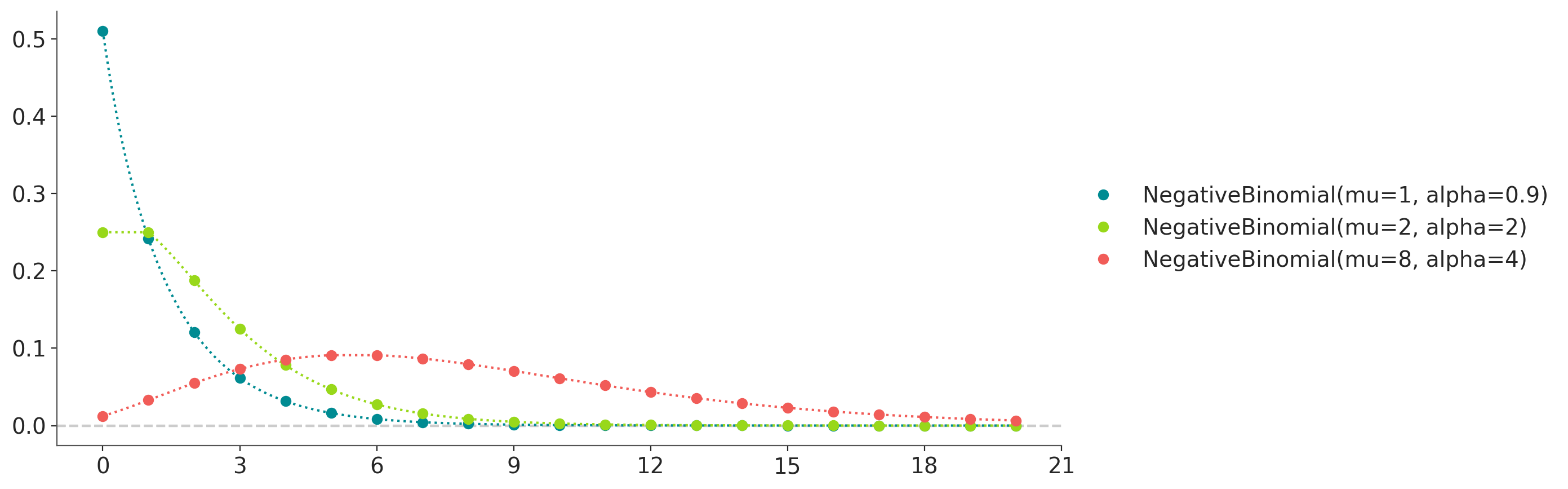
class preliz.distributions.zi_binomial.ZeroInflatedBinomial(psi=None, n=None, p=None)[source]#

Zero-inflated Binomial distribution.

The pmf of this distribution is

\[\begin{split}f(x \mid \psi, n, p) = \left\{ \begin{array}{l} (1-\psi) + \psi (1-p)^{n}, \text{if } x = 0 \\ \psi {n \choose x} p^x (1-p)^{n-x}, \text{if } x=1,2,3,\ldots,n \end{array} \right.\end{split}\]

(Source code, png, hires.png, pdf)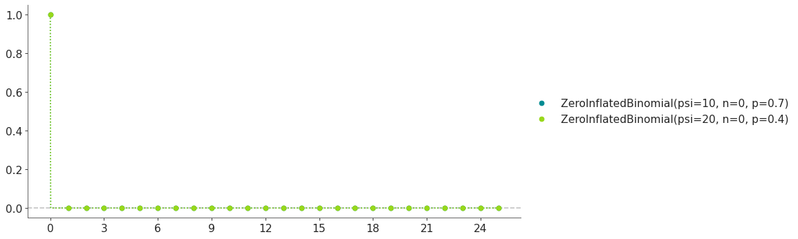

Support	$x \in \mathbb{N}_0$
Mean	$\psi n p$
Variance	$\psi n p (1 - p) + n^2 p^2 (\psi - \psi^2)$

Parameters:

psi (float) – Expected proportion of Binomial variates (0 < psi < 1)
n (int) – Number of Bernoulli trials (n >= 0).
p (float) – Probability of success in each trial (0 < p < 1).

cdf(x)[source]#

Cumulative distribution function.

Parameters:: x (array_like) – Values on which to evaluate the cdf

entropy()[source]#: Entropy.

eti(mass=None, fmt='.2f')#

Equal-tailed interval containing mass.

Parameters:

mass (float) – Probability mass in the interval. Defaults to None,
used. (which results in the value of rcParams["stats.ci_prob"] being)
fmt (str) – fmt used to represent results using f-string fmt for floats. Default to “.2f” i.e. 2 digits after the decimal point. Use “none” for no format.

hdi(mass=None, fmt='.2f')#

Highest density interval containing mass.

Parameters:

mass (float) – Probability mass in the interval. Defaults to None,
used. (which results in the value of rcParams["stats.ci_prob"] being)
fmt (str) – fmt used to represent results using f-string fmt for floats. Default to “.2f” i.e. 2 digits after the decimal point. Use “none” for no format.

isf(x)#

Inverse survival function (inverse of sf).

Parameters:: x (array_like) – Values on which to evaluate the inverse of the sf

kurtosis()[source]#: Excess kurtosis.

lmoment1()[source]#: L-moment1 (mean).

lmoment2()[source]#: L-moment2 (l-scale).

lmoment3()[source]#: L-moment3 (l-skewness). This the ratio of L-moment3 to L-moment2.

lmoment4()[source]#: L-moment4 (l-kurtosis). This the ratio of L-moment4 to L-moment2.

lmoments(types='1234')#

Compute L-moments of the distribution.

Parameters:: types (str) – The type of moments to compute. Default is ‘1234’ where ‘1’ = L-moment1 (mean), ‘2’ = L-moment2 (l-scale), ‘3’ = L-moment3 (l-skewness), and ‘4’ = L-moment4 (l-kurtosis). To compute the standard deviation use ‘d’ Valid combinations are any subset of ‘1234’.

logcdf(x)#

Log cumulative distribution function.

Parameters:: x (array_like) – Values on which to evaluate the logcdf

logpdf(x)[source]#

Log probability density/mass function.

Parameters:: x (array_like) – Values on which to evaluate the logpdf

logsf(x)#

Log survival function log(1 - cdf).

Parameters:: x (array_like) – Values on which to evaluate the logsf

mean()[source]#: Mean.

median()[source]#: Median.

mode()[source]#: Mode.

moments(types='mvsk')#

Compute moments of the distribution.

It can also return the standard deviation

Parameters:: types (str) – The type of moments to compute. Default is ‘mvsk’ where ‘m’ = mean, ‘v’ = variance, ‘s’ = skewness, and ‘k’ = kurtosis. To compute the standard deviation use ‘d’ Valid combinations are any subset of ‘mvdsk’.

pdf(x)[source]#

Probability density/mass function.

Parameters:: x (array_like) – Values on which to evaluate the pdf

plot_cdf(moments=None, pointinterval=False, interval=None, levels=None, support='restricted', legend='legend', figsize=None, ax=None, **kwargs)#

Plot the cumulative distribution function.

Parameters:

moments (str) – Compute moments. Use any combination of the strings m, d, v, s or k for the mean (μ), standard deviation (σ), variance (σ²), skew (γ) or kurtosis (κ) respectively. Other strings will be ignored. Defaults to None.
pointinterval (bool) – Whether to include a plot of the quantiles. Defaults to False. If True the default is to plot the median and two interquantiles ranges.
interval (str) – Type of interval. Available options are highest density interval “hdi” (default), equal tailed interval “eti” or intervals defined by arbitrary “quantiles”. Defaults to the value in rcParams[“stats.ci_kind”].
levels (list) – Mass of the intervals. For hdi or eti the number of elements should be 2 or 1. For quantiles the number of elements should be 5, 3, 1 or 0 (in this last case nothing will be plotted).
support (str:) – If full use the finite end-points to set the limits of the plot. For unbounded end-points or if restricted use the 0.001 and 0.999 quantiles to set the limits.
legend (str) – Whether to include a string with the distribution and its parameter as a "legend" a "title" or not include them None.
figsize (tuple) – Size of the figure
ax (matplotlib axes)
kwargs (keyword arguments) – Additional keyword arguments passed to matplotlib plot function. For example, color, alpha, linewidth, etc.

plot_interactive(kind='pdf', xy_lim='both', pointinterval=True, interval=None, levels=None, figsize=None)#

Interactive exploration of distributions parameters.

Parameters:

kind (str:) – Type of plot. Available options are pdf, cdf and ppf.
xy_lim (str or tuple) – Set the limits of the x-axis and/or y-axis. Defaults to “both”, the limits of both axis are fixed. Use “auto” for automatic rescaling of x-axis and y-axis. Or set them manually by passing a tuple of 4 elements, the first two for x-axis, the last two for y-axis. The tuple can have None.
pointinterval (bool) – Whether to include a plot of the quantiles. Defaults to False. If True the default is to plot the median and two interquantiles ranges.
interval (str) – Type of interval. Available options are highest density interval “hdi” (default), equal tailed interval “eti” or intervals defined by arbitrary “quantiles”. Defaults to the value in rcParams[“stats.ci_kind”].
levels (list) – Mass of the intervals. For hdi or eti the number of elements should be 2 or 1. For quantiles the number of elements should be 5, 3, 1 or 0 (in this last case nothing will be plotted).
figsize (tuple) – Size of the figure

plot_isf(moments=None, pointinterval=False, interval=None, levels=None, legend='legend', figsize=None, ax=None, **kwargs)#

Plot the inverse survival function.

Parameters:

moments (str) – Compute moments. Use any combination of the strings m, d, v, s or k for the mean (μ), standard deviation (σ), variance (σ²), skew (γ) or kurtosis (κ) respectively. Other strings will be ignored. Defaults to None.
pointinterval (bool) – Whether to include a plot of the quantiles. Defaults to False. If True the default is to plot the median and two interquantiles ranges.
interval (str) – Type of interval. Available options are highest density interval “hdi” (default), equal tailed interval “eti” or intervals defined by arbitrary “quantiles”. Defaults to the value in rcParams[“stats.ci_kind”].
levels (list) – Mass of the intervals. For hdi or eti the number of elements should be 2 or 1. For quantiles the number of elements should be 5, 3, 1 or 0 (in this last case nothing will be plotted).
legend (str) – Whether to include a string with the distribution and its parameter as a "legend" a "title" or not include them None.
figsize (tuple) – Size of the figure
ax (matplotlib axes)

plot_pdf(moments=None, pointinterval=False, interval=None, levels=None, support='restricted', baseline=True, legend='legend', figsize=None, ax=None, **kwargs)#

Plot the pdf (continuous) or pmf (discrete).

Parameters:

moments (str) – Compute moments. Use any combination of the strings m, d, v, s or k for the mean (μ), standard deviation (σ), variance (σ²), skew (γ) or kurtosis (κ) respectively. Other strings will be ignored. Defaults to None.
pointinterval (bool) – Whether to include a plot of the quantiles. Defaults to False. If True the default is to plot the median and two interquantiles ranges.
interval (str) – Type of interval. Available options are highest density interval “hdi” (default), equal tailed interval “eti” or intervals defined by arbitrary “quantiles”. Defaults to the value in rcParams[“stats.ci_kind”].
levels (list) – Mass of the intervals. For hdi or eti the number of elements should be 2 or 1. For quantiles the number of elements should be 5, 3, 1 or 0 (in this last case nothing will be plotted).
support (str:) – If full use the finite end-points to set the limits of the plot. For unbounded end-points or if restricted use the 0.001 and 0.999 quantiles to set the limits.
baseline (bool) – Whether to include a horizontal line at y=0.
legend (str) – Whether to include a string with the distribution and its parameter as a "legend" a "title" or not include them None.
figsize (tuple) – Size of the figure
ax (matplotlib axes)
kwargs (keyword arguments) – Additional keyword arguments passed to matplotlib plot function. For example, color, alpha, linewidth, etc.

plot_ppf(moments=None, pointinterval=False, interval=None, levels=None, legend='legend', figsize=None, ax=None, **kwargs)#

Plot the quantile function.

Parameters:

moments (str) – Compute moments. Use any combination of the strings m, d, v, s or k for the mean (μ), standard deviation (σ), variance (σ²), skew (γ) or kurtosis (κ) respectively. Other strings will be ignored. Defaults to None.
pointinterval (bool) – Whether to include a plot of the quantiles. Defaults to False. If True the default is to plot the median and two interquantiles ranges.
interval (str) – Type of interval. Available options are highest density interval “hdi” (default), equal tailed interval “eti” or intervals defined by arbitrary “quantiles”. Defaults to the value in rcParams[“stats.ci_kind”].
levels (list) – Mass of the intervals. For hdi or eti the number of elements should be 2 or 1. For quantiles the number of elements should be 5, 3, 1 or 0 (in this last case nothing will be plotted).
legend (str) – Whether to include a string with the distribution and its parameter as a "legend" a "title" or not include them None.
figsize (tuple) – Size of the figure
ax (matplotlib axes)

plot_sf(moments=None, pointinterval=False, interval=None, levels=None, support='restricted', legend='legend', figsize=None, ax=None, **kwargs)#

Plot the survival distribution function (1 - CDF).

Parameters:

moments (str) – Compute moments. Use any combination of the strings m, d, v, s or k for the mean (μ), standard deviation (σ), variance (σ²), skew (γ) or kurtosis (κ) respectively. Other strings will be ignored. Defaults to None.
pointinterval (bool) – Whether to include a plot of the quantiles. Defaults to False. If True the default is to plot the median and two interquantiles ranges.
interval (str) – Type of interval. Available options are highest density interval “hdi” (default), equal tailed interval “eti” or intervals defined by arbitrary “quantiles”. Defaults to the value in rcParams[“stats.ci_kind”].
levels (list) – Mass of the intervals. For hdi or eti the number of elements should be 2 or 1. For quantiles the number of elements should be 5, 3, 1 or 0 (in this last case nothing will be plotted).
support (str:) – If full use the finite end-points to set the limits of the plot. For unbounded end-points or if restricted use the 0.001 and 0.999 quantiles to set the limits.
legend (str) – Whether to include a string with the distribution and its parameter as a "legend" a "title" or not include them None.
figsize (tuple) – Size of the figure
ax (matplotlib axes)
kwargs (keyword arguments) – Additional keyword arguments passed to matplotlib plot function. For example, color, alpha, linewidth, etc.

ppf(q)[source]#

Percent point function (inverse of cdf).

Parameters:: x (array_like) – Values on which to evaluate the inverse of the cdf

rvs(size=None, random_state=None)[source]#

Random sample.

Parameters:

size (int or tuple of ints, optional) – Defining number of random variates. Defaults to 1.
random_state ({None, int, numpy.random.Generator, numpy.random.RandomState}) – Defaults to None

sf(x)#

Survival function (1 - cdf).

Parameters:: x (array_like) – Values on which to evaluate the sf

skewness()[source]#: Skewness.

std()[source]#: Standard deviation.

summary(mass=None, interval=None, fmt='.2f')#

Namedtuple with the mean, median, sd, and lower and upper bounds.

Parameters:

mass (float) – Probability mass for the equal-tailed interval. Defaults to None,
used. (which results in the value of rcParams["stats.ci_prob"] being)
interval (str or list-like) – Type of interval. Available options are highest density interval “hdi”, equal tailed interval “eti” or arbitrary interval defined by a list-like object with a pair of values. Defaults to the value in rcParams[“stats.ci_kind”].
fmt (str) – fmt used to represent results using f-string fmt for floats. Default to “.2f” i.e. 2 digits after the decimal point.

to_bambi(**kwargs)#

Convert the PreliZ distribution to a Bambi Prior.

kwargsPyMC distributions properties: kwargs are used to specify properties such as shape or dims

Return type:: Bambi Prior

to_pymc(name=None, **kwargs)#

Convert the PreliZ distribution to a PyMC distribution.

namestr: Name of PyMC distribution. Needed if inside Model context
kwargsPyMC distributions properties: kwargs are used to specify properties such as shape or dims

Return type:: PyMC distribution

var()[source]#: Variance.

xvals(support, n_points=None)#

Provide x values in the support of the distribution.

This is useful for example when plotting.

Parameters:

support (str) – Available options are “full” or “restricted”. If “full” the values will cover the entire support of the distribution if the boundary is finite, or the quantiles 0.0001 or 0.9999, if infinite. If “restricted” the values will cover the quantile 0.0001 to 0.9999.
n_points (int) – Number of values to return. Defaults to 1000 for continuous distributions and 200 for discrete ones. For discrete distributions the returned values may be fewer than n_points if the actual number of discrete values in the support of the distribution is smaller than n_points.

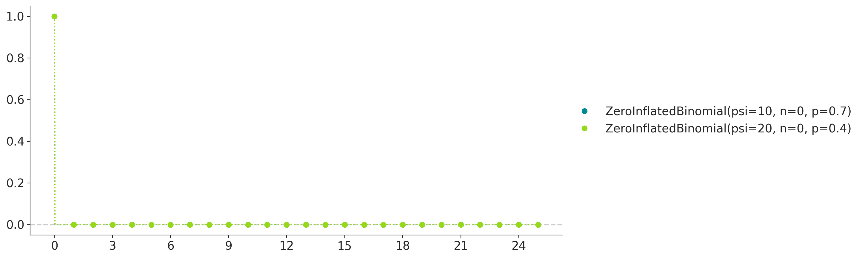
class preliz.distributions.zi_negativebinomial.ZeroInflatedNegativeBinomial(psi=None, mu=None, alpha=None, p=None, n=None)[source]#

Zero-Inflated Negative binomial distribution.

The Zero-inflated version of the Negative Binomial (NB). The NB distribution describes a Poisson random variable whose rate parameter is gamma distributed. The pmf of this distribution is

\[\begin{split}f(x \mid \psi, \mu, \alpha) = \left\{ \begin{array}{l} (1-\psi) + \psi \left ( \frac{\alpha}{\alpha+\mu} \right) ^\alpha, \text{if } x = 0 \\ \psi \frac{\Gamma(x+\alpha)}{x! \Gamma(\alpha)} \left ( \frac{\alpha}{\mu+\alpha} \right)^\alpha \left( \frac{\mu}{\mu+\alpha} \right)^x, \text{if } x=1,2,3,\ldots \end{array} \right.\end{split}\]

(Source code, png, hires.png, pdf)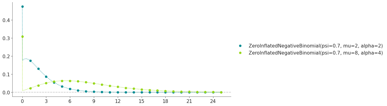

The zero inflated negative binomial distribution can be parametrized either in terms of mu and alpha, or in terms of n and p. The link between the parametrizations is given by

\[\begin{split}\mu &= \frac{n(1-p)}{p} \\ \alpha &= n\end{split}\]

Parameters:

psi (float) – Expected proportion of NegativeBinomial variates (0 < psi < 1)
mu (float) – Poisson distribution parameter (mu > 0).
alpha (float) – Gamma distribution parameter (alpha > 0).
p (float) – Alternative probability of success in each trial (0 < p < 1).
n (float) – Alternative number of target success trials (n > 0)

cdf(x)[source]#

Cumulative distribution function.

Parameters:: x (array_like) – Values on which to evaluate the cdf

entropy()[source]#: Entropy.

eti(mass=None, fmt='.2f')#

Equal-tailed interval containing mass.

Parameters:

mass (float) – Probability mass in the interval. Defaults to None,
used. (which results in the value of rcParams["stats.ci_prob"] being)
fmt (str) – fmt used to represent results using f-string fmt for floats. Default to “.2f” i.e. 2 digits after the decimal point. Use “none” for no format.

hdi(mass=None, fmt='.2f')#

Highest density interval containing mass.

Parameters:

mass (float) – Probability mass in the interval. Defaults to None,
used. (which results in the value of rcParams["stats.ci_prob"] being)
fmt (str) – fmt used to represent results using f-string fmt for floats. Default to “.2f” i.e. 2 digits after the decimal point. Use “none” for no format.

isf(x)#

Inverse survival function (inverse of sf).

Parameters:: x (array_like) – Values on which to evaluate the inverse of the sf

kurtosis()[source]#: Excess kurtosis.

lmoment1()[source]#: L-moment1 (mean).

lmoment2()[source]#: L-moment2 (l-scale).

lmoment3()[source]#: L-moment3 (l-skewness). This the ratio of L-moment3 to L-moment2.

lmoment4()[source]#: L-moment4 (l-kurtosis). This the ratio of L-moment4 to L-moment2.

lmoments(types='1234')#

Compute L-moments of the distribution.

Parameters:: types (str) – The type of moments to compute. Default is ‘1234’ where ‘1’ = L-moment1 (mean), ‘2’ = L-moment2 (l-scale), ‘3’ = L-moment3 (l-skewness), and ‘4’ = L-moment4 (l-kurtosis). To compute the standard deviation use ‘d’ Valid combinations are any subset of ‘1234’.

logcdf(x)#

Log cumulative distribution function.

Parameters:: x (array_like) – Values on which to evaluate the logcdf

logpdf(x)[source]#

Log probability density/mass function.

Parameters:: x (array_like) – Values on which to evaluate the logpdf

logsf(x)#

Log survival function log(1 - cdf).

Parameters:: x (array_like) – Values on which to evaluate the logsf

mean()[source]#: Mean.

median()[source]#: Median.

mode()[source]#: Mode.

moments(types='mvsk')#

Compute moments of the distribution.

It can also return the standard deviation

Parameters:: types (str) – The type of moments to compute. Default is ‘mvsk’ where ‘m’ = mean, ‘v’ = variance, ‘s’ = skewness, and ‘k’ = kurtosis. To compute the standard deviation use ‘d’ Valid combinations are any subset of ‘mvdsk’.

pdf(x)[source]#

Probability density/mass function.

Parameters:: x (array_like) – Values on which to evaluate the pdf

plot_cdf(moments=None, pointinterval=False, interval=None, levels=None, support='restricted', legend='legend', figsize=None, ax=None, **kwargs)#

Plot the cumulative distribution function.

Parameters:

moments (str) – Compute moments. Use any combination of the strings m, d, v, s or k for the mean (μ), standard deviation (σ), variance (σ²), skew (γ) or kurtosis (κ) respectively. Other strings will be ignored. Defaults to None.
pointinterval (bool) – Whether to include a plot of the quantiles. Defaults to False. If True the default is to plot the median and two interquantiles ranges.
interval (str) – Type of interval. Available options are highest density interval “hdi” (default), equal tailed interval “eti” or intervals defined by arbitrary “quantiles”. Defaults to the value in rcParams[“stats.ci_kind”].
levels (list) – Mass of the intervals. For hdi or eti the number of elements should be 2 or 1. For quantiles the number of elements should be 5, 3, 1 or 0 (in this last case nothing will be plotted).
support (str:) – If full use the finite end-points to set the limits of the plot. For unbounded end-points or if restricted use the 0.001 and 0.999 quantiles to set the limits.
legend (str) – Whether to include a string with the distribution and its parameter as a "legend" a "title" or not include them None.
figsize (tuple) – Size of the figure
ax (matplotlib axes)
kwargs (keyword arguments) – Additional keyword arguments passed to matplotlib plot function. For example, color, alpha, linewidth, etc.

plot_interactive(kind='pdf', xy_lim='both', pointinterval=True, interval=None, levels=None, figsize=None)#

Interactive exploration of distributions parameters.

Parameters:

kind (str:) – Type of plot. Available options are pdf, cdf and ppf.
xy_lim (str or tuple) – Set the limits of the x-axis and/or y-axis. Defaults to “both”, the limits of both axis are fixed. Use “auto” for automatic rescaling of x-axis and y-axis. Or set them manually by passing a tuple of 4 elements, the first two for x-axis, the last two for y-axis. The tuple can have None.
pointinterval (bool) – Whether to include a plot of the quantiles. Defaults to False. If True the default is to plot the median and two interquantiles ranges.
interval (str) – Type of interval. Available options are highest density interval “hdi” (default), equal tailed interval “eti” or intervals defined by arbitrary “quantiles”. Defaults to the value in rcParams[“stats.ci_kind”].
levels (list) – Mass of the intervals. For hdi or eti the number of elements should be 2 or 1. For quantiles the number of elements should be 5, 3, 1 or 0 (in this last case nothing will be plotted).
figsize (tuple) – Size of the figure

plot_isf(moments=None, pointinterval=False, interval=None, levels=None, legend='legend', figsize=None, ax=None, **kwargs)#

Plot the inverse survival function.

Parameters:

moments (str) – Compute moments. Use any combination of the strings m, d, v, s or k for the mean (μ), standard deviation (σ), variance (σ²), skew (γ) or kurtosis (κ) respectively. Other strings will be ignored. Defaults to None.
pointinterval (bool) – Whether to include a plot of the quantiles. Defaults to False. If True the default is to plot the median and two interquantiles ranges.
interval (str) – Type of interval. Available options are highest density interval “hdi” (default), equal tailed interval “eti” or intervals defined by arbitrary “quantiles”. Defaults to the value in rcParams[“stats.ci_kind”].
levels (list) – Mass of the intervals. For hdi or eti the number of elements should be 2 or 1. For quantiles the number of elements should be 5, 3, 1 or 0 (in this last case nothing will be plotted).
legend (str) – Whether to include a string with the distribution and its parameter as a "legend" a "title" or not include them None.
figsize (tuple) – Size of the figure
ax (matplotlib axes)

plot_pdf(moments=None, pointinterval=False, interval=None, levels=None, support='restricted', baseline=True, legend='legend', figsize=None, ax=None, **kwargs)#

Plot the pdf (continuous) or pmf (discrete).

Parameters:

moments (str) – Compute moments. Use any combination of the strings m, d, v, s or k for the mean (μ), standard deviation (σ), variance (σ²), skew (γ) or kurtosis (κ) respectively. Other strings will be ignored. Defaults to None.
pointinterval (bool) – Whether to include a plot of the quantiles. Defaults to False. If True the default is to plot the median and two interquantiles ranges.
interval (str) – Type of interval. Available options are highest density interval “hdi” (default), equal tailed interval “eti” or intervals defined by arbitrary “quantiles”. Defaults to the value in rcParams[“stats.ci_kind”].
levels (list) – Mass of the intervals. For hdi or eti the number of elements should be 2 or 1. For quantiles the number of elements should be 5, 3, 1 or 0 (in this last case nothing will be plotted).
support (str:) – If full use the finite end-points to set the limits of the plot. For unbounded end-points or if restricted use the 0.001 and 0.999 quantiles to set the limits.
baseline (bool) – Whether to include a horizontal line at y=0.
legend (str) – Whether to include a string with the distribution and its parameter as a "legend" a "title" or not include them None.
figsize (tuple) – Size of the figure
ax (matplotlib axes)
kwargs (keyword arguments) – Additional keyword arguments passed to matplotlib plot function. For example, color, alpha, linewidth, etc.

plot_ppf(moments=None, pointinterval=False, interval=None, levels=None, legend='legend', figsize=None, ax=None, **kwargs)#

Plot the quantile function.

Parameters:

moments (str) – Compute moments. Use any combination of the strings m, d, v, s or k for the mean (μ), standard deviation (σ), variance (σ²), skew (γ) or kurtosis (κ) respectively. Other strings will be ignored. Defaults to None.
pointinterval (bool) – Whether to include a plot of the quantiles. Defaults to False. If True the default is to plot the median and two interquantiles ranges.
interval (str) – Type of interval. Available options are highest density interval “hdi” (default), equal tailed interval “eti” or intervals defined by arbitrary “quantiles”. Defaults to the value in rcParams[“stats.ci_kind”].
levels (list) – Mass of the intervals. For hdi or eti the number of elements should be 2 or 1. For quantiles the number of elements should be 5, 3, 1 or 0 (in this last case nothing will be plotted).
legend (str) – Whether to include a string with the distribution and its parameter as a "legend" a "title" or not include them None.
figsize (tuple) – Size of the figure
ax (matplotlib axes)

plot_sf(moments=None, pointinterval=False, interval=None, levels=None, support='restricted', legend='legend', figsize=None, ax=None, **kwargs)#

Plot the survival distribution function (1 - CDF).

Parameters:

moments (str) – Compute moments. Use any combination of the strings m, d, v, s or k for the mean (μ), standard deviation (σ), variance (σ²), skew (γ) or kurtosis (κ) respectively. Other strings will be ignored. Defaults to None.
pointinterval (bool) – Whether to include a plot of the quantiles. Defaults to False. If True the default is to plot the median and two interquantiles ranges.
interval (str) – Type of interval. Available options are highest density interval “hdi” (default), equal tailed interval “eti” or intervals defined by arbitrary “quantiles”. Defaults to the value in rcParams[“stats.ci_kind”].
levels (list) – Mass of the intervals. For hdi or eti the number of elements should be 2 or 1. For quantiles the number of elements should be 5, 3, 1 or 0 (in this last case nothing will be plotted).
support (str:) – If full use the finite end-points to set the limits of the plot. For unbounded end-points or if restricted use the 0.001 and 0.999 quantiles to set the limits.
legend (str) – Whether to include a string with the distribution and its parameter as a "legend" a "title" or not include them None.
figsize (tuple) – Size of the figure
ax (matplotlib axes)
kwargs (keyword arguments) – Additional keyword arguments passed to matplotlib plot function. For example, color, alpha, linewidth, etc.

ppf(q)[source]#

Percent point function (inverse of cdf).

Parameters:: x (array_like) – Values on which to evaluate the inverse of the cdf

rvs(size=None, random_state=None)[source]#

Random sample.

Parameters:

size (int or tuple of ints, optional) – Defining number of random variates. Defaults to 1.
random_state ({None, int, numpy.random.Generator, numpy.random.RandomState}) – Defaults to None

sf(x)#

Survival function (1 - cdf).

Parameters:: x (array_like) – Values on which to evaluate the sf

skewness()[source]#: Skewness.

std()[source]#: Standard deviation.

summary(mass=None, interval=None, fmt='.2f')#

Namedtuple with the mean, median, sd, and lower and upper bounds.

Parameters:

mass (float) – Probability mass for the equal-tailed interval. Defaults to None,
used. (which results in the value of rcParams["stats.ci_prob"] being)
interval (str or list-like) – Type of interval. Available options are highest density interval “hdi”, equal tailed interval “eti” or arbitrary interval defined by a list-like object with a pair of values. Defaults to the value in rcParams[“stats.ci_kind”].
fmt (str) – fmt used to represent results using f-string fmt for floats. Default to “.2f” i.e. 2 digits after the decimal point.

to_bambi(**kwargs)#

Convert the PreliZ distribution to a Bambi Prior.

kwargsPyMC distributions properties: kwargs are used to specify properties such as shape or dims

Return type:: Bambi Prior

to_pymc(name=None, **kwargs)#

Convert the PreliZ distribution to a PyMC distribution.

namestr: Name of PyMC distribution. Needed if inside Model context
kwargsPyMC distributions properties: kwargs are used to specify properties such as shape or dims

Return type:: PyMC distribution

var()[source]#: Variance.

xvals(support, n_points=None)#

Provide x values in the support of the distribution.

This is useful for example when plotting.

Parameters:

support (str) – Available options are “full” or “restricted”. If “full” the values will cover the entire support of the distribution if the boundary is finite, or the quantiles 0.0001 or 0.9999, if infinite. If “restricted” the values will cover the quantile 0.0001 to 0.9999.
n_points (int) – Number of values to return. Defaults to 1000 for continuous distributions and 200 for discrete ones. For discrete distributions the returned values may be fewer than n_points if the actual number of discrete values in the support of the distribution is smaller than n_points.

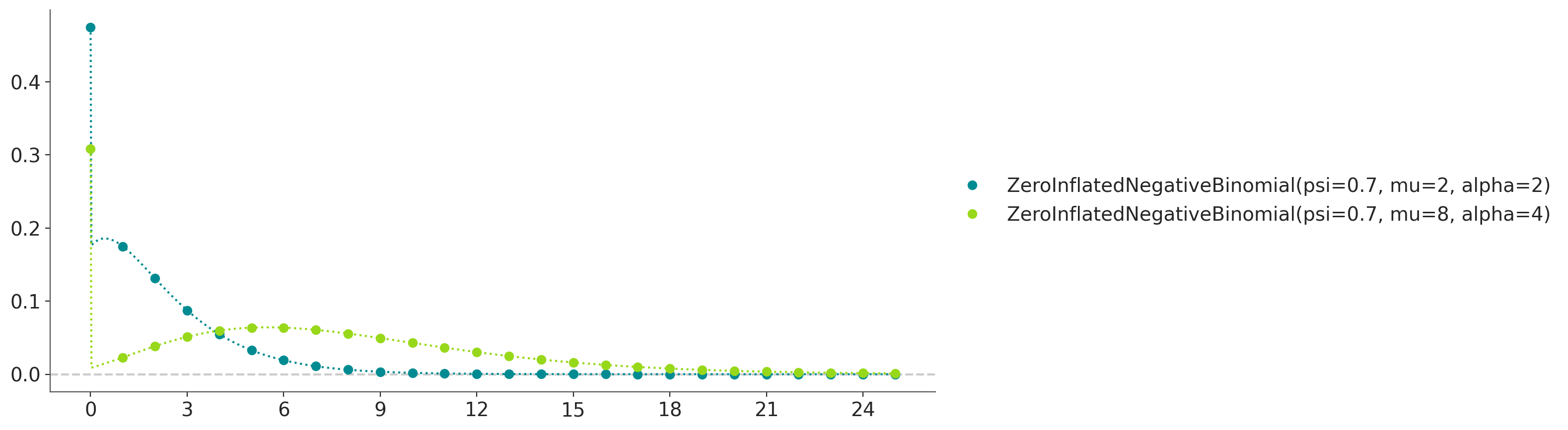
class preliz.distributions.zi_poisson.ZeroInflatedPoisson(psi=None, mu=None)[source]#

Zero-inflated Poisson distribution.

Often used to model the number of events occurring in a fixed period of time when the times at which events occur are independent. The pmf of this distribution is

\[\begin{split}f(x \mid \psi, \mu) = \left\{ \begin{array}{l} (1-\psi) + \psi e^{-\mu}, \text{if } x = 0 \\ \psi \frac{e^{-\mu}\mu^x}{x!}, \text{if } x=1,2,3,\ldots \end{array} \right.\end{split}\]

(Source code, png, hires.png, pdf)

Support	$x \in \mathbb{N}_0$
Mean	$\psi \mu$
Variance	$\psi \mu (1+(1-\psi) \mu$

Parameters:

psi (float) – Expected proportion of Poisson variates (0 < psi < 1)
mu (float) – Expected number of occurrences during the given interval (mu >= 0).

cdf(x)[source]#

Cumulative distribution function.

Parameters:: x (array_like) – Values on which to evaluate the cdf

entropy()[source]#: Entropy.

eti(mass=None, fmt='.2f')#

Equal-tailed interval containing mass.

Parameters:

mass (float) – Probability mass in the interval. Defaults to None,
used. (which results in the value of rcParams["stats.ci_prob"] being)
fmt (str) – fmt used to represent results using f-string fmt for floats. Default to “.2f” i.e. 2 digits after the decimal point. Use “none” for no format.

hdi(mass=None, fmt='.2f')#

Highest density interval containing mass.

Parameters:

mass (float) – Probability mass in the interval. Defaults to None,
used. (which results in the value of rcParams["stats.ci_prob"] being)
fmt (str) – fmt used to represent results using f-string fmt for floats. Default to “.2f” i.e. 2 digits after the decimal point. Use “none” for no format.

isf(x)#

Inverse survival function (inverse of sf).

Parameters:: x (array_like) – Values on which to evaluate the inverse of the sf

kurtosis()[source]#: Excess kurtosis.

lmoment1()[source]#: L-moment1 (mean).

lmoment2()[source]#: L-moment2 (l-scale).

lmoment3()[source]#: L-moment3 (l-skewness). This the ratio of L-moment3 to L-moment2.

lmoment4()[source]#: L-moment4 (l-kurtosis). This the ratio of L-moment4 to L-moment2.

lmoments(types='1234')#

Compute L-moments of the distribution.

Parameters:: types (str) – The type of moments to compute. Default is ‘1234’ where ‘1’ = L-moment1 (mean), ‘2’ = L-moment2 (l-scale), ‘3’ = L-moment3 (l-skewness), and ‘4’ = L-moment4 (l-kurtosis). To compute the standard deviation use ‘d’ Valid combinations are any subset of ‘1234’.

logcdf(x)#

Log cumulative distribution function.

Parameters:: x (array_like) – Values on which to evaluate the logcdf

logpdf(x)[source]#

Log probability density/mass function.

Parameters:: x (array_like) – Values on which to evaluate the logpdf

logsf(x)#

Log survival function log(1 - cdf).

Parameters:: x (array_like) – Values on which to evaluate the logsf

mean()[source]#: Mean.

median()[source]#: Median.

mode()[source]#: Mode.

moments(types='mvsk')#

Compute moments of the distribution.

It can also return the standard deviation

Parameters:: types (str) – The type of moments to compute. Default is ‘mvsk’ where ‘m’ = mean, ‘v’ = variance, ‘s’ = skewness, and ‘k’ = kurtosis. To compute the standard deviation use ‘d’ Valid combinations are any subset of ‘mvdsk’.

pdf(x)[source]#

Probability density/mass function.

Parameters:: x (array_like) – Values on which to evaluate the pdf

plot_cdf(moments=None, pointinterval=False, interval=None, levels=None, support='restricted', legend='legend', figsize=None, ax=None, **kwargs)#

Plot the cumulative distribution function.

Parameters:

moments (str) – Compute moments. Use any combination of the strings m, d, v, s or k for the mean (μ), standard deviation (σ), variance (σ²), skew (γ) or kurtosis (κ) respectively. Other strings will be ignored. Defaults to None.
pointinterval (bool) – Whether to include a plot of the quantiles. Defaults to False. If True the default is to plot the median and two interquantiles ranges.
interval (str) – Type of interval. Available options are highest density interval “hdi” (default), equal tailed interval “eti” or intervals defined by arbitrary “quantiles”. Defaults to the value in rcParams[“stats.ci_kind”].
levels (list) – Mass of the intervals. For hdi or eti the number of elements should be 2 or 1. For quantiles the number of elements should be 5, 3, 1 or 0 (in this last case nothing will be plotted).
support (str:) – If full use the finite end-points to set the limits of the plot. For unbounded end-points or if restricted use the 0.001 and 0.999 quantiles to set the limits.
legend (str) – Whether to include a string with the distribution and its parameter as a "legend" a "title" or not include them None.
figsize (tuple) – Size of the figure
ax (matplotlib axes)
kwargs (keyword arguments) – Additional keyword arguments passed to matplotlib plot function. For example, color, alpha, linewidth, etc.

plot_interactive(kind='pdf', xy_lim='both', pointinterval=True, interval=None, levels=None, figsize=None)#

Interactive exploration of distributions parameters.

Parameters:

kind (str:) – Type of plot. Available options are pdf, cdf and ppf.
xy_lim (str or tuple) – Set the limits of the x-axis and/or y-axis. Defaults to “both”, the limits of both axis are fixed. Use “auto” for automatic rescaling of x-axis and y-axis. Or set them manually by passing a tuple of 4 elements, the first two for x-axis, the last two for y-axis. The tuple can have None.
pointinterval (bool) – Whether to include a plot of the quantiles. Defaults to False. If True the default is to plot the median and two interquantiles ranges.
interval (str) – Type of interval. Available options are highest density interval “hdi” (default), equal tailed interval “eti” or intervals defined by arbitrary “quantiles”. Defaults to the value in rcParams[“stats.ci_kind”].
levels (list) – Mass of the intervals. For hdi or eti the number of elements should be 2 or 1. For quantiles the number of elements should be 5, 3, 1 or 0 (in this last case nothing will be plotted).
figsize (tuple) – Size of the figure

plot_isf(moments=None, pointinterval=False, interval=None, levels=None, legend='legend', figsize=None, ax=None, **kwargs)#

Plot the inverse survival function.

Parameters:

moments (str) – Compute moments. Use any combination of the strings m, d, v, s or k for the mean (μ), standard deviation (σ), variance (σ²), skew (γ) or kurtosis (κ) respectively. Other strings will be ignored. Defaults to None.
pointinterval (bool) – Whether to include a plot of the quantiles. Defaults to False. If True the default is to plot the median and two interquantiles ranges.
interval (str) – Type of interval. Available options are highest density interval “hdi” (default), equal tailed interval “eti” or intervals defined by arbitrary “quantiles”. Defaults to the value in rcParams[“stats.ci_kind”].
levels (list) – Mass of the intervals. For hdi or eti the number of elements should be 2 or 1. For quantiles the number of elements should be 5, 3, 1 or 0 (in this last case nothing will be plotted).
legend (str) – Whether to include a string with the distribution and its parameter as a "legend" a "title" or not include them None.
figsize (tuple) – Size of the figure
ax (matplotlib axes)

plot_pdf(moments=None, pointinterval=False, interval=None, levels=None, support='restricted', baseline=True, legend='legend', figsize=None, ax=None, **kwargs)#

Plot the pdf (continuous) or pmf (discrete).

Parameters:

moments (str) – Compute moments. Use any combination of the strings m, d, v, s or k for the mean (μ), standard deviation (σ), variance (σ²), skew (γ) or kurtosis (κ) respectively. Other strings will be ignored. Defaults to None.
pointinterval (bool) – Whether to include a plot of the quantiles. Defaults to False. If True the default is to plot the median and two interquantiles ranges.
interval (str) – Type of interval. Available options are highest density interval “hdi” (default), equal tailed interval “eti” or intervals defined by arbitrary “quantiles”. Defaults to the value in rcParams[“stats.ci_kind”].
levels (list) – Mass of the intervals. For hdi or eti the number of elements should be 2 or 1. For quantiles the number of elements should be 5, 3, 1 or 0 (in this last case nothing will be plotted).
support (str:) – If full use the finite end-points to set the limits of the plot. For unbounded end-points or if restricted use the 0.001 and 0.999 quantiles to set the limits.
baseline (bool) – Whether to include a horizontal line at y=0.
legend (str) – Whether to include a string with the distribution and its parameter as a "legend" a "title" or not include them None.
figsize (tuple) – Size of the figure
ax (matplotlib axes)
kwargs (keyword arguments) – Additional keyword arguments passed to matplotlib plot function. For example, color, alpha, linewidth, etc.

plot_ppf(moments=None, pointinterval=False, interval=None, levels=None, legend='legend', figsize=None, ax=None, **kwargs)#

Plot the quantile function.

Parameters:

moments (str) – Compute moments. Use any combination of the strings m, d, v, s or k for the mean (μ), standard deviation (σ), variance (σ²), skew (γ) or kurtosis (κ) respectively. Other strings will be ignored. Defaults to None.
pointinterval (bool) – Whether to include a plot of the quantiles. Defaults to False. If True the default is to plot the median and two interquantiles ranges.
interval (str) – Type of interval. Available options are highest density interval “hdi” (default), equal tailed interval “eti” or intervals defined by arbitrary “quantiles”. Defaults to the value in rcParams[“stats.ci_kind”].
levels (list) – Mass of the intervals. For hdi or eti the number of elements should be 2 or 1. For quantiles the number of elements should be 5, 3, 1 or 0 (in this last case nothing will be plotted).
legend (str) – Whether to include a string with the distribution and its parameter as a "legend" a "title" or not include them None.
figsize (tuple) – Size of the figure
ax (matplotlib axes)

plot_sf(moments=None, pointinterval=False, interval=None, levels=None, support='restricted', legend='legend', figsize=None, ax=None, **kwargs)#

Plot the survival distribution function (1 - CDF).

Parameters:

moments (str) – Compute moments. Use any combination of the strings m, d, v, s or k for the mean (μ), standard deviation (σ), variance (σ²), skew (γ) or kurtosis (κ) respectively. Other strings will be ignored. Defaults to None.
pointinterval (bool) – Whether to include a plot of the quantiles. Defaults to False. If True the default is to plot the median and two interquantiles ranges.
interval (str) – Type of interval. Available options are highest density interval “hdi” (default), equal tailed interval “eti” or intervals defined by arbitrary “quantiles”. Defaults to the value in rcParams[“stats.ci_kind”].
levels (list) – Mass of the intervals. For hdi or eti the number of elements should be 2 or 1. For quantiles the number of elements should be 5, 3, 1 or 0 (in this last case nothing will be plotted).
support (str:) – If full use the finite end-points to set the limits of the plot. For unbounded end-points or if restricted use the 0.001 and 0.999 quantiles to set the limits.
legend (str) – Whether to include a string with the distribution and its parameter as a "legend" a "title" or not include them None.
figsize (tuple) – Size of the figure
ax (matplotlib axes)
kwargs (keyword arguments) – Additional keyword arguments passed to matplotlib plot function. For example, color, alpha, linewidth, etc.

ppf(q)[source]#

Percent point function (inverse of cdf).

Parameters:: x (array_like) – Values on which to evaluate the inverse of the cdf

rvs(size=None, random_state=None)[source]#

Random sample.

Parameters:

size (int or tuple of ints, optional) – Defining number of random variates. Defaults to 1.
random_state ({None, int, numpy.random.Generator, numpy.random.RandomState}) – Defaults to None

sf(x)#

Survival function (1 - cdf).

Parameters:: x (array_like) – Values on which to evaluate the sf

skewness()[source]#: Skewness.

std()[source]#: Standard deviation.

summary(mass=None, interval=None, fmt='.2f')#

Namedtuple with the mean, median, sd, and lower and upper bounds.

Parameters:

mass (float) – Probability mass for the equal-tailed interval. Defaults to None,
used. (which results in the value of rcParams["stats.ci_prob"] being)
interval (str or list-like) – Type of interval. Available options are highest density interval “hdi”, equal tailed interval “eti” or arbitrary interval defined by a list-like object with a pair of values. Defaults to the value in rcParams[“stats.ci_kind”].
fmt (str) – fmt used to represent results using f-string fmt for floats. Default to “.2f” i.e. 2 digits after the decimal point.

to_bambi(**kwargs)#

Convert the PreliZ distribution to a Bambi Prior.

kwargsPyMC distributions properties: kwargs are used to specify properties such as shape or dims

Return type:: Bambi Prior

to_pymc(name=None, **kwargs)#

Convert the PreliZ distribution to a PyMC distribution.

namestr: Name of PyMC distribution. Needed if inside Model context
kwargsPyMC distributions properties: kwargs are used to specify properties such as shape or dims

Return type:: PyMC distribution

var()[source]#: Variance.

xvals(support, n_points=None)#

Provide x values in the support of the distribution.

This is useful for example when plotting.

Parameters:

support (str) – Available options are “full” or “restricted”. If “full” the values will cover the entire support of the distribution if the boundary is finite, or the quantiles 0.0001 or 0.9999, if infinite. If “restricted” the values will cover the quantile 0.0001 to 0.9999.
n_points (int) – Number of values to return. Defaults to 1000 for continuous distributions and 200 for discrete ones. For discrete distributions the returned values may be fewer than n_points if the actual number of discrete values in the support of the distribution is smaller than n_points.

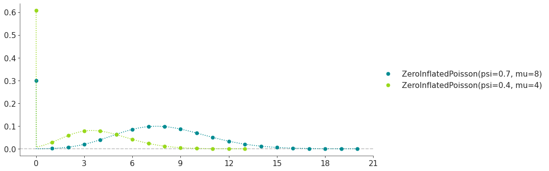
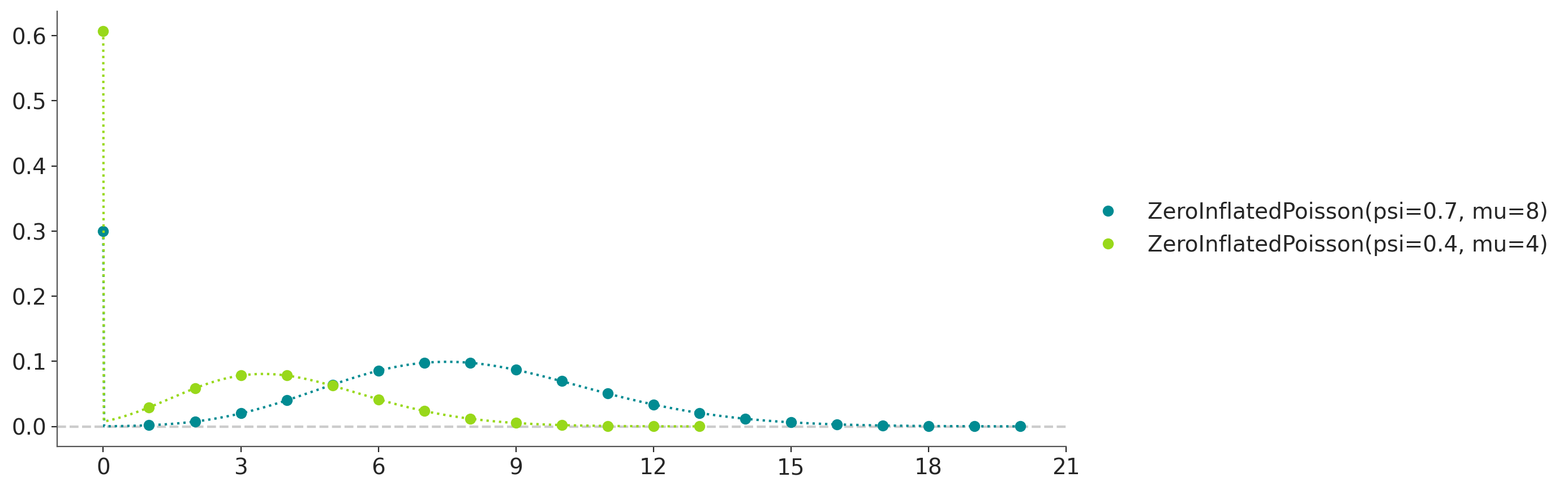
`preliz.distributions.continuous_multivariate`#

Continuous multivariate probability distributions.

class preliz.distributions.continuous_multivariate.Dirichlet(alpha=None)[source]#

Dirichlet distribution.

\[f(\mathbf{x}|\mathbf{a}) = \frac{\Gamma(\sum_{i=1}^k a_i)}{\prod_{i=1}^k \Gamma(a_i)} \prod_{i=1}^k x_i^{a_i - 1}\]

(Source code)

Support	$x_i \in (0, 1)$ for $i \in \{1, \ldots, K\}$ such that $\sum x_i = 1$
Mean	$\dfrac{a_i}{\sum a_i}$
Variance	$\dfrac{a_i - \sum a_0}{a_0^2 (a_0 + 1)}$ where $a_0 = \sum a_i$

Parameters:: alpha (array of floats) – Concentration parameter (alpha > 0).

entropy()#: Entropy of the distribution.

logpdf(x)#

Logarithm of the probability density function at x.

Parameters:: x (array_like) – Values on which to evaluate the logpdf

mean()#: Mean of the distribution.

pdf(x)#

Probability density function at x.

Parameters:: x (array_like) – Values on which to evaluate the pdf

plot_cdf(pointinterval=False, interval=None, levels=None, support='full', legend='title', figsize=None, ax=None)[source]#

Plot the cumulative distribution function.

Parameters:

pointinterval (bool) – Whether to include a plot of the quantiles. Defaults to False. If True the default is to plot the median and two interquantile ranges.
interval (str) – Type of interval. Available options are highest density interval “hdi”,
"quantiles". (equal tailed interval "eti" or intervals defined by arbitrary)
rcParams["stats.ci_kind"]. (Defaults to the value in)
levels (list) – Mass of the intervals. For hdi or eti the number of elements should be 2 or 1. For quantiles the number of elements should be 5, 3, 1 or 0 (in this last case nothing will be plotted).
support (str:) – If full use the finite end-points to set the limits of the plot. For unbounded end-points or if restricted use the 0.001 and 0.999 quantiles to set the limits.
legend (str) – Whether to include a string with the distribution and its parameter as a "title" or not include them None.
figsize (tuple) – Size of the figure
ax (matplotlib axis) – Axis to plot on

Returns:

ax

Return type:

matplotlib axis

plot_interactive(kind='pdf', xy_lim='both', pointinterval=True, interval=None, levels=None, baseline=True, legend='title', figsize=None)[source]#

Interactive exploration of parameters.

Parameters:

kind (str:) – Type of plot. Available options are pdf, cdf and ppf.
xy_lim (str or tuple) – Set the limits of the x-axis and/or y-axis. Defaults to “both”, the limits of both axes are fixed for all subplots. Use “auto” for automatic rescaling of x-axis and y-axis. Or set them manually by passing a tuple of 4 elements, the first two for x-axis, the last two for y-axis. The tuple can have None.
pointinterval (bool) – Whether to include a plot of the quantiles. Defaults to False. If True the default is to plot the median and two inter-quantiles ranges.
interval (str) – Type of interval. Available options are the highest density interval “hdi”, equal tailed interval “eti” or intervals defined by arbitrary “quantiles”.
levels (list) – Mass of the intervals. For hdi or eti the number of elements should be 2 or 1. For quantiles the number of elements should be 5, 3, 1 or 0 (in this last case nothing will be plotted).
baseline (bool) – Whether to include a baseline in the plot. Defaults to True. Only applicable for pdf plots.
legend (str) – Whether to include a string with the distribution and its parameter as a "title" or not include them None.
figsize (tuple) – Size of the figure

plot_isf(pointinterval=False, interval=None, levels=None, legend='title', figsize=None, ax=None)[source]#

Plot the inverse survival function.

Parameters:

pointinterval (bool) – Whether to include a plot of the quantiles. Defaults to False. If True the default is to plot the median and two interquantile ranges.
interval (str) – Type of interval. Available options are highest density interval “hdi”,
"quantiles". (equal tailed interval "eti" or intervals defined by arbitrary)
rcParams["stats.ci_kind"]. (Defaults to the value in)
levels (list) – Mass of the intervals. For hdi or eti the number of elements should be 2 or 1. For quantiles the number of elements should be 5, 3, 1 or 0 (in this last case nothing will be plotted).
legend (str) – Whether to include a string with the distribution and its parameter as a "title" or not include them None.
figsize (tuple) – Size of the figure
ax (matplotlib axis) – Axis to plot on

Returns:

ax

Return type:

matplotlib axis

plot_pdf(marginals=True, pointinterval=False, interval=None, levels=None, support='full', baseline=True, legend='title', figsize=None, ax=None)[source]#

Plot the pdf of the marginals or the joint pdf of the simplex.

The joint representation is only available for a dirichlet with an alpha of length 3.

Parameters:

marginals (True) – Defaults to True, plot the marginal distributions, if False plot the joint distribution (only valid for an alpha of length 3).
pointinterval (bool) – Whether to include a plot of the quantiles. Defaults to False. If True the default is to plot the median and two interquantile ranges.
interval (str) – Type of interval. Available options are highest density interval “hdi”,
"quantiles". (equal tailed interval "eti" or intervals defined by arbitrary)
rcParams["stats.ci_kind"]. (Defaults to the value in)
levels (list) – Mass of the intervals. For hdi or eti the number of elements should be 2 or 1. For quantiles the number of elements should be 5, 3, 1 or 0 (in this last case nothing will be plotted).
support (str:) – If full use the finite end-points to set the limits of the plot. For unbounded end-points or if restricted use the 0.001 and 0.999 quantiles to set the limits.
baseline (bool) – Whether to include a baseline in the plot. Defaults to True. Only used when marginals=True.
legend (str) – Whether to include a string with the distribution and its parameter as a "title" or not include them None.
figsize (tuple) – Size of the figure
ax (matplotlib axis) – Axis to plot on

Returns:

ax

Return type:

matplotlib axis

plot_ppf(pointinterval=False, interval=None, levels=None, legend='title', figsize=None, ax=None)[source]#

Plot the quantile function.

Parameters:

pointinterval (bool) – Whether to include a plot of the quantiles. Defaults to False. If True the default is to plot the median and two interquantile ranges.
interval (str) – Type of interval. Available options are highest density interval “hdi”,
"quantiles". (equal tailed interval "eti" or intervals defined by arbitrary)
rcParams["stats.ci_kind"]. (Defaults to the value in)
levels (list) – Mass of the intervals. For hdi or eti the number of elements should be 2 or 1. For quantiles the number of elements should be 5, 3, 1 or 0 (in this last case nothing will be plotted).
legend (str) – Whether to include a string with the distribution and its parameter as a "title" or not include them None.
figsize (tuple) – Size of the figure
ax (matplotlib axis) – Axis to plot on

Returns:

ax

Return type:

matplotlib axis

plot_sf(pointinterval=False, interval=None, levels=None, support='full', legend='title', figsize=None, ax=None)[source]#

Plot the survival function (1 - CDF).

Parameters:

pointinterval (bool) – Whether to include a plot of the quantiles. Defaults to False. If True the default is to plot the median and two interquantile ranges.
interval (str) – Type of interval. Available options are highest density interval “hdi”,
"quantiles". (equal tailed interval "eti" or intervals defined by arbitrary)
rcParams["stats.ci_kind"]. (Defaults to the value in)
levels (list) – Mass of the intervals. For hdi or eti the number of elements should be 2 or 1. For quantiles the number of elements should be 5, 3, 1 or 0 (in this last case nothing will be plotted).
support (str:) – If full use the finite end-points to set the limits of the plot. For unbounded end-points or if restricted use the 0.001 and 0.999 quantiles to set the limits.
legend (str) – Whether to include a string with the distribution and its parameter as a "title" or not include them None.
figsize (tuple) – Size of the figure
ax (matplotlib axis) – Axis to plot on

Returns:

ax

Return type:

matplotlib axis

rvs(*args, **kwds)#

Random sample.

Parameters:

size (int or tuple of ints, optional) – Defining number of random variates. Defaults to 1.
random_state ({None, int, numpy.random.Generator, numpy.random.RandomState}) – Defaults to None

summary()#: Namedtuple with the mean, and standard deviation of the distribution.

var()#: Variance of the distribution.

xvals(support)#

Provide x values in the support of the distribution.

This is useful for example when plotting.

Parameters:: support (str) – Available options are “full” or “restricted”.

class preliz.distributions.continuous_multivariate.MvNormal(mu=None, cov=None, tau=None)[source]#

Multivariate Normal distribution.

\[f(x \mid \mu, T) = \frac{|T|^{1/2}}{(2\pi)^{k/2}} \exp\left\{ -\frac{1}{2} (x-\mu)^{\prime} T (x-\mu) \right\}\]

(Source code, png, hires.png, pdf)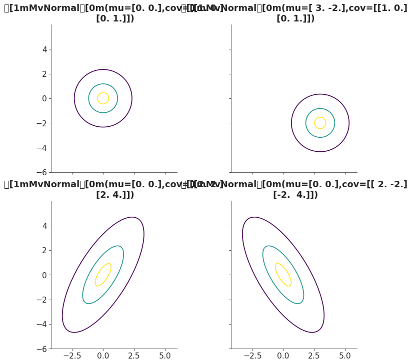

Support	$x \in \mathbb{R}^k$
Mean	$\mu$
Variance	$T^{-1}$

MvNormal distribution has 2 alternative parameterizations. In terms of the mean and the covariance matrix, or in terms of the mean and the precision matrix.

The link between the 2 alternatives is given by

\[T = \Sigma^{-1}\]

Parameters:

mu (array of floats) – Vector of means.
cov (array of floats, optional) – Covariance matrix.
tau (array of floats, optional) – Precision matrix.

entropy()#: Entropy of the distribution.

logpdf(x)#

Logarithm of the probability density function at x.

Parameters:: x (array_like) – Values on which to evaluate the logpdf

mean()#: Mean of the distribution.

pdf(x)#

Probability density function at x.

Parameters:: x (array_like) – Values on which to evaluate the pdf

plot_cdf(pointinterval=False, interval=None, levels=None, support='full', legend='title', figsize=None, ax=None)[source]#

Plot the cumulative distribution function.

Parameters:

pointinterval (bool) – Whether to include a plot of the quantiles. Defaults to False. If True the default is to plot the median and two interquantiles ranges.
interval (str) – Type of interval. Available options are highest density interval “hdi”,
"quantiles". (equal tailed interval "eti" or intervals defined by arbitrary)
rcParams["stats.ci_kind"]. (Defaults to the value in)
levels (list) – Mass of the intervals. For hdi or eti the number of elements should be 2 or 1. For quantiles the number of elements should be 5, 3, 1 or 0 (in this last case nothing will be plotted).
support (str:) – If full use the finite end-points to set the limits of the plot. For unbounded end-points or if restricted use the 0.001 and 0.999 quantiles to set the limits.
legend (str) – Whether to include a string with the distribution and its parameter as a "title" or not include them None.
figsize (tuple) – Size of the figure
ax (matplotlib axis) – Axis to plot on

Returns:

ax

Return type:

matplotlib axis

plot_interactive(kind='pdf', xy_lim='both', pointinterval=True, interval=None, levels=None, baseline=True, legend='title', figsize=None)[source]#

Interactive exploration of parameters.

Parameters:

kind (str:) – Type of plot. Available options are pdf, cdf and ppf.
xy_lim (str or tuple) – Set the limits of the x-axis and/or y-axis. Defaults to “both”, the limits of both axes are fixed for all subplots. Use “auto” for automatic rescaling of x-axis and y-axis. Or set them manually by passing a tuple of 4 elements, the first two for x-axis, the last two for y-axis. The tuple can have None.
pointinterval (bool) – Whether to include a plot of the quantiles. Defaults to False. If True the default is to plot the median and two inter-quantiles ranges.
interval (str) – Type of interval. Available options are the highest density interval “hdi”, equal tailed interval “eti” or intervals defined by arbitrary “quantiles”. Defaults to the value in rcParams[“stats.ci_kind”].
levels (list) – Mass of the intervals. For hdi or eti the number of elements should be 2 or 1. For quantiles the number of elements should be 5, 3, 1 or 0 (in this last case nothing will be plotted).
baseline (bool) – Whether to include a baseline in the plot. Defaults to True. Only applicable for pdf plots.
legend (str) – Whether to include a string with the distribution and its parameter as a "title" or not include them None.
figsize (tuple) – Size of the figure

plot_isf(pointinterval=False, interval=None, levels=None, legend='title', figsize=None, ax=None)[source]#

Plot the inverse survival function.

Parameters:

pointinterval (bool) – Whether to include a plot of the quantiles. Defaults to False. If True the default is to plot the median and two interquantiles ranges.
interval (str) – Type of interval. Available options are highest density interval “hdi”,
"quantiles". (equal tailed interval "eti" or intervals defined by arbitrary)
rcParams["stats.ci_kind"]. (Defaults to the value in)
levels (list) – Mass of the intervals. For hdi or eti the number of elements should be 2 or 1. For quantiles the number of elements should be 5, 3, 1 or 0 (in this last case nothing will be plotted).
legend (str) – Whether to include a string with the distribution and its parameter as a "title" or not include them None.
figsize (tuple) – Size of the figure
ax (matplotlib axis) – Axis to plot on

Returns:

ax

Return type:

matplotlib axis

plot_pdf(marginals=True, pointinterval=False, interval=None, levels=None, support='full', baseline=True, legend='title', figsize=None, ax=None)[source]#

Plot the pdf of the marginals or the joint pdf.

The joint representation is only available for a 2D Multivariate Normal.

Parameters:

marginals (True) – Defaults to True, plot the marginal distributions, if False plot the joint distribution (only valid for a bivariate normal).
pointinterval (bool) – Whether to include a plot of the quantiles. Defaults to False. If True the default is to plot the median and two interquantiles ranges.
interval (str) – Type of interval. Available options are highest density interval “hdi”,
"quantiles". (equal tailed interval "eti" or intervals defined by arbitrary)
rcParams["stats.ci_kind"]. (Defaults to the value in)
levels (list) – Mass of the intervals. For hdi or eti the number of elements should be 2 or 1. For quantiles the number of elements should be 5, 3, 1 or 0 (in this last case nothing will be plotted).
support (str:) – If full use the finite end-points to set the limits of the plot. For unbounded end-points or if restricted use the 0.001 and 0.999 quantiles to set the limits.
baseline (bool) – Whether to include a baseline in the plot. Defaults to True. Only used when marginals=True.
legend (str) – Whether to include a string with the distribution and its parameter as a "title" or not include them None.
figsize (tuple) – Size of the figure
ax (matplotlib axis) – Axis to plot on

Returns:

ax

Return type:

matplotlib axis

plot_ppf(pointinterval=False, interval=None, levels=None, legend='title', figsize=None, ax=None)[source]#

Plot the quantile function.

Parameters:

pointinterval (bool) – Whether to include a plot of the quantiles. Defaults to False. If True the default is to plot the median and two interquantiles ranges.
interval (str) – Type of interval. Available options are highest density interval “hdi”,
"quantiles". (equal tailed interval "eti" or intervals defined by arbitrary)
rcParams["stats.ci_kind"]. (Defaults to the value in)
levels (list) – Mass of the intervals. For hdi or eti the number of elements should be 2 or 1. For quantiles the number of elements should be 5, 3, 1 or 0 (in this last case nothing will be plotted).
legend (str) – Whether to include a string with the distribution and its parameter as a "title" or not include them None.
figsize (tuple) – Size of the figure
ax (matplotlib axis) – Axis to plot on

Returns:

ax

Return type:

matplotlib axis

plot_sf(pointinterval=False, interval=None, levels=None, support='full', legend='title', figsize=None, ax=None)[source]#

Plot the survival function (1 - CDF).

Parameters:

pointinterval (bool) – Whether to include a plot of the quantiles. Defaults to False. If True the default is to plot the median and two interquantiles ranges.
interval (str) – Type of interval. Available options are highest density interval “hdi”,
"quantiles". (equal tailed interval "eti" or intervals defined by arbitrary)
rcParams["stats.ci_kind"]. (Defaults to the value in)
levels (list) – Mass of the intervals. For hdi or eti the number of elements should be 2 or 1. For quantiles the number of elements should be 5, 3, 1 or 0 (in this last case nothing will be plotted).
support (str:) – If full use the finite end-points to set the limits of the plot. For unbounded end-points or if restricted use the 0.001 and 0.999 quantiles to set the limits.
legend (str) – Whether to include a string with the distribution and its parameter as a "title" or not include them None.
figsize (tuple) – Size of the figure
ax (matplotlib axis) – Axis to plot on

Returns:

ax

Return type:

matplotlib axis

rvs(*args, **kwds)#

Random sample.

Parameters:

size (int or tuple of ints, optional) – Defining number of random variates. Defaults to 1.
random_state ({None, int, numpy.random.Generator, numpy.random.RandomState}) – Defaults to None

summary()#: Namedtuple with the mean, and standard deviation of the distribution.

var()#: Variance of the distribution.

xvals(support)#

Provide x values in the support of the distribution.

This is useful for example when plotting.

Parameters:: support (str) – Available options are “full” or “restricted”.

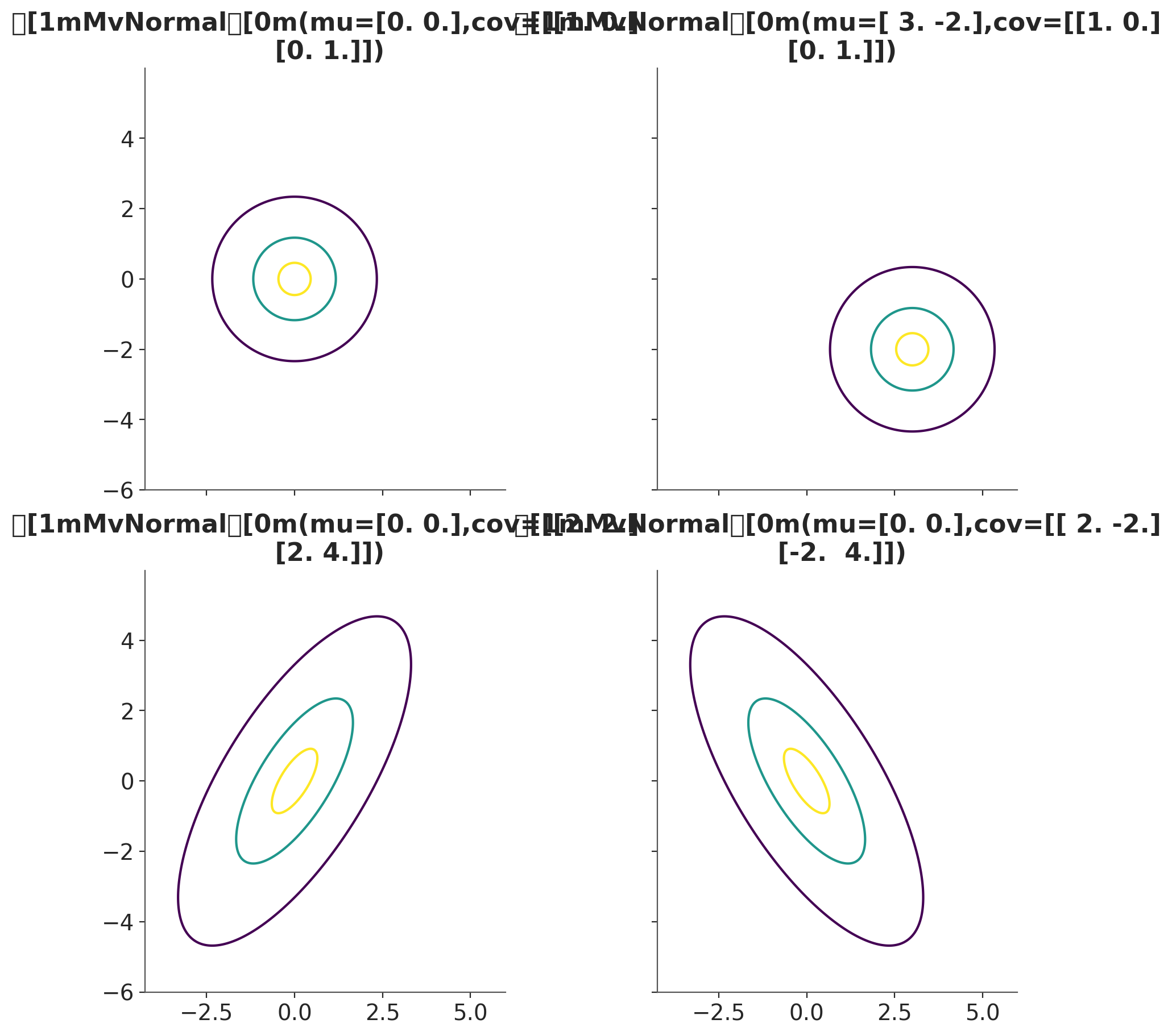
`preliz.distributions`#

class preliz.distributions.censored.Censored(dist, lower=None, upper=None, **kwargs)[source]#

Censored distribution.

This is not a distribution per se, but a modifier of univariate distributions.

Given a base distribution with cumulative distribution function (CDF) and probability density mass/function (PDF). The pdf of a Censored distribution is:

\[\begin{split}\begin{cases} 0 & \text{for } x < \text{lower}, \\ \text{CDF}(\text{lower}) & \text{for } x = \text{lower}, \\ \text{PDF}(x) & \text{for } \text{lower} < x < \text{upper}, \\ 1-\text{CDF}(\text{upper}) & \text {for } x = \text{upper}, \\ 0 & \text{for } x > \text{upper}, \end{cases}\end{split}\]

(Source code, png, hires.png, pdf)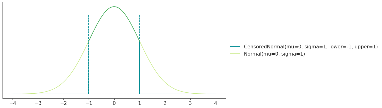

Parameters:

dist (PreliZ distribution) – Univariate PreliZ distribution which will be censored.
lower (float or int) – Lower (left) censoring point. Use np.inf for no censoring.
upper (float or int) – Upper (right) censoring point. Use np.inf for no censoring.

cdf(x)[source]#

Cumulative distribution function.

Parameters:: x (array_like) – Values on which to evaluate the cdf

entropy()[source]#: Entropy.

eti(mass=None, fmt='.2f')#

Equal-tailed interval containing mass.

Parameters:

mass (float) – Probability mass in the interval. Defaults to None,
used. (which results in the value of rcParams["stats.ci_prob"] being)
fmt (str) – fmt used to represent results using f-string fmt for floats. Default to “.2f” i.e. 2 digits after the decimal point. Use “none” for no format.

hdi(mass=None, fmt='.2f')#

Highest density interval containing mass.

Parameters:

mass (float) – Probability mass in the interval. Defaults to None,
used. (which results in the value of rcParams["stats.ci_prob"] being)
fmt (str) – fmt used to represent results using f-string fmt for floats. Default to “.2f” i.e. 2 digits after the decimal point. Use “none” for no format.

isf(x)#

Inverse survival function (inverse of sf).

Parameters:: x (array_like) – Values on which to evaluate the inverse of the sf

kurtosis()[source]#: Excess kurtosis.

lmoment1()#: L-moment1 (mean).

lmoment2()#: L-moment2 (l-scale).

lmoment3()#: L-moment3 (l-skewness). This the ratio of L-moment3 to L-moment2.

lmoment4()#: L-moment4 (l-kurtosis). This the ratio of L-moment4 to L-moment2.

lmoments(types='1234')#

Compute L-moments of the distribution.

Parameters:: types (str) – The type of moments to compute. Default is ‘1234’ where ‘1’ = L-moment1 (mean), ‘2’ = L-moment2 (l-scale), ‘3’ = L-moment3 (l-skewness), and ‘4’ = L-moment4 (l-kurtosis). To compute the standard deviation use ‘d’ Valid combinations are any subset of ‘1234’.

logcdf(x)#

Log cumulative distribution function.

Parameters:: x (array_like) – Values on which to evaluate the logcdf

logpdf(x)[source]#

Log probability density/mass function.

Parameters:: x (array_like) – Values on which to evaluate the logpdf

logsf(x)#

Log survival function log(1 - cdf).

Parameters:: x (array_like) – Values on which to evaluate the logsf

mean()[source]#: Mean.

median()[source]#: Median.

mode()[source]#: Mode.

moments(types='mvsk')#

Compute moments of the distribution.

It can also return the standard deviation

Parameters:: types (str) – The type of moments to compute. Default is ‘mvsk’ where ‘m’ = mean, ‘v’ = variance, ‘s’ = skewness, and ‘k’ = kurtosis. To compute the standard deviation use ‘d’ Valid combinations are any subset of ‘mvdsk’.

pdf(x)[source]#

Probability density/mass function.

Parameters:: x (array_like) – Values on which to evaluate the pdf

plot_cdf(moments=None, pointinterval=False, interval=None, levels=None, support='restricted', legend='legend', figsize=None, ax=None, **kwargs)#

Plot the cumulative distribution function.

Parameters:

moments (str) – Compute moments. Use any combination of the strings m, d, v, s or k for the mean (μ), standard deviation (σ), variance (σ²), skew (γ) or kurtosis (κ) respectively. Other strings will be ignored. Defaults to None.
pointinterval (bool) – Whether to include a plot of the quantiles. Defaults to False. If True the default is to plot the median and two interquantiles ranges.
interval (str) – Type of interval. Available options are highest density interval “hdi” (default), equal tailed interval “eti” or intervals defined by arbitrary “quantiles”. Defaults to the value in rcParams[“stats.ci_kind”].
levels (list) – Mass of the intervals. For hdi or eti the number of elements should be 2 or 1. For quantiles the number of elements should be 5, 3, 1 or 0 (in this last case nothing will be plotted).
support (str:) – If full use the finite end-points to set the limits of the plot. For unbounded end-points or if restricted use the 0.001 and 0.999 quantiles to set the limits.
legend (str) – Whether to include a string with the distribution and its parameter as a "legend" a "title" or not include them None.
figsize (tuple) – Size of the figure
ax (matplotlib axes)
kwargs (keyword arguments) – Additional keyword arguments passed to matplotlib plot function. For example, color, alpha, linewidth, etc.

plot_interactive(kind='pdf', xy_lim='both', pointinterval=True, interval=None, levels=None, figsize=None)#

Interactive exploration of distributions parameters.

Parameters:

kind (str:) – Type of plot. Available options are pdf, cdf and ppf.
xy_lim (str or tuple) – Set the limits of the x-axis and/or y-axis. Defaults to “both”, the limits of both axis are fixed. Use “auto” for automatic rescaling of x-axis and y-axis. Or set them manually by passing a tuple of 4 elements, the first two for x-axis, the last two for y-axis. The tuple can have None.
pointinterval (bool) – Whether to include a plot of the quantiles. Defaults to False. If True the default is to plot the median and two interquantiles ranges.
interval (str) – Type of interval. Available options are highest density interval “hdi” (default), equal tailed interval “eti” or intervals defined by arbitrary “quantiles”. Defaults to the value in rcParams[“stats.ci_kind”].
levels (list) – Mass of the intervals. For hdi or eti the number of elements should be 2 or 1. For quantiles the number of elements should be 5, 3, 1 or 0 (in this last case nothing will be plotted).
figsize (tuple) – Size of the figure

plot_isf(moments=None, pointinterval=False, interval=None, levels=None, legend='legend', figsize=None, ax=None, **kwargs)#

Plot the inverse survival function.

Parameters:

moments (str) – Compute moments. Use any combination of the strings m, d, v, s or k for the mean (μ), standard deviation (σ), variance (σ²), skew (γ) or kurtosis (κ) respectively. Other strings will be ignored. Defaults to None.
pointinterval (bool) – Whether to include a plot of the quantiles. Defaults to False. If True the default is to plot the median and two interquantiles ranges.
interval (str) – Type of interval. Available options are highest density interval “hdi” (default), equal tailed interval “eti” or intervals defined by arbitrary “quantiles”. Defaults to the value in rcParams[“stats.ci_kind”].
levels (list) – Mass of the intervals. For hdi or eti the number of elements should be 2 or 1. For quantiles the number of elements should be 5, 3, 1 or 0 (in this last case nothing will be plotted).
legend (str) – Whether to include a string with the distribution and its parameter as a "legend" a "title" or not include them None.
figsize (tuple) – Size of the figure
ax (matplotlib axes)

plot_pdf(moments=None, pointinterval=False, interval=None, levels=None, support='restricted', baseline=True, legend='legend', figsize=None, ax=None, **kwargs)#

Plot the pdf (continuous) or pmf (discrete).

Parameters:

moments (str) – Compute moments. Use any combination of the strings m, d, v, s or k for the mean (μ), standard deviation (σ), variance (σ²), skew (γ) or kurtosis (κ) respectively. Other strings will be ignored. Defaults to None.
pointinterval (bool) – Whether to include a plot of the quantiles. Defaults to False. If True the default is to plot the median and two interquantiles ranges.
interval (str) – Type of interval. Available options are highest density interval “hdi” (default), equal tailed interval “eti” or intervals defined by arbitrary “quantiles”. Defaults to the value in rcParams[“stats.ci_kind”].
levels (list) – Mass of the intervals. For hdi or eti the number of elements should be 2 or 1. For quantiles the number of elements should be 5, 3, 1 or 0 (in this last case nothing will be plotted).
support (str:) – If full use the finite end-points to set the limits of the plot. For unbounded end-points or if restricted use the 0.001 and 0.999 quantiles to set the limits.
baseline (bool) – Whether to include a horizontal line at y=0.
legend (str) – Whether to include a string with the distribution and its parameter as a "legend" a "title" or not include them None.
figsize (tuple) – Size of the figure
ax (matplotlib axes)
kwargs (keyword arguments) – Additional keyword arguments passed to matplotlib plot function. For example, color, alpha, linewidth, etc.

plot_ppf(moments=None, pointinterval=False, interval=None, levels=None, legend='legend', figsize=None, ax=None, **kwargs)#

Plot the quantile function.

Parameters:

moments (str) – Compute moments. Use any combination of the strings m, d, v, s or k for the mean (μ), standard deviation (σ), variance (σ²), skew (γ) or kurtosis (κ) respectively. Other strings will be ignored. Defaults to None.
pointinterval (bool) – Whether to include a plot of the quantiles. Defaults to False. If True the default is to plot the median and two interquantiles ranges.
interval (str) – Type of interval. Available options are highest density interval “hdi” (default), equal tailed interval “eti” or intervals defined by arbitrary “quantiles”. Defaults to the value in rcParams[“stats.ci_kind”].
levels (list) – Mass of the intervals. For hdi or eti the number of elements should be 2 or 1. For quantiles the number of elements should be 5, 3, 1 or 0 (in this last case nothing will be plotted).
legend (str) – Whether to include a string with the distribution and its parameter as a "legend" a "title" or not include them None.
figsize (tuple) – Size of the figure
ax (matplotlib axes)

plot_sf(moments=None, pointinterval=False, interval=None, levels=None, support='restricted', legend='legend', figsize=None, ax=None, **kwargs)#

Plot the survival distribution function (1 - CDF).

Parameters:

moments (str) – Compute moments. Use any combination of the strings m, d, v, s or k for the mean (μ), standard deviation (σ), variance (σ²), skew (γ) or kurtosis (κ) respectively. Other strings will be ignored. Defaults to None.
pointinterval (bool) – Whether to include a plot of the quantiles. Defaults to False. If True the default is to plot the median and two interquantiles ranges.
interval (str) – Type of interval. Available options are highest density interval “hdi” (default), equal tailed interval “eti” or intervals defined by arbitrary “quantiles”. Defaults to the value in rcParams[“stats.ci_kind”].
levels (list) – Mass of the intervals. For hdi or eti the number of elements should be 2 or 1. For quantiles the number of elements should be 5, 3, 1 or 0 (in this last case nothing will be plotted).
support (str:) – If full use the finite end-points to set the limits of the plot. For unbounded end-points or if restricted use the 0.001 and 0.999 quantiles to set the limits.
legend (str) – Whether to include a string with the distribution and its parameter as a "legend" a "title" or not include them None.
figsize (tuple) – Size of the figure
ax (matplotlib axes)
kwargs (keyword arguments) – Additional keyword arguments passed to matplotlib plot function. For example, color, alpha, linewidth, etc.

ppf(q)[source]#

Percent point function (inverse of cdf).

Parameters:: x (array_like) – Values on which to evaluate the inverse of the cdf

rvs(size=None, random_state=None)[source]#

Random sample.

Parameters:

size (int or tuple of ints, optional) – Defining number of random variates. Defaults to 1.
random_state ({None, int, numpy.random.Generator, numpy.random.RandomState}) – Defaults to None

sf(x)#

Survival function (1 - cdf).

Parameters:: x (array_like) – Values on which to evaluate the sf

skewness()[source]#: Skewness.

std()[source]#: Standard deviation.

summary(mass=None, interval=None, fmt='.2f')#

Namedtuple with the mean, median, sd, and lower and upper bounds.

Parameters:

mass (float) – Probability mass for the equal-tailed interval. Defaults to None,
used. (which results in the value of rcParams["stats.ci_prob"] being)
interval (str or list-like) – Type of interval. Available options are highest density interval “hdi”, equal tailed interval “eti” or arbitrary interval defined by a list-like object with a pair of values. Defaults to the value in rcParams[“stats.ci_kind”].
fmt (str) – fmt used to represent results using f-string fmt for floats. Default to “.2f” i.e. 2 digits after the decimal point.

to_bambi(**kwargs)#

Convert the PreliZ distribution to a Bambi Prior.

kwargsPyMC distributions properties: kwargs are used to specify properties such as shape or dims

Return type:: Bambi Prior

to_pymc(name=None, **kwargs)#

Convert the PreliZ distribution to a PyMC distribution.

namestr: Name of PyMC distribution. Needed if inside Model context
kwargsPyMC distributions properties: kwargs are used to specify properties such as shape or dims

Return type:: PyMC distribution

var()[source]#: Variance.

xvals(support, n_points=None)#

Provide x values in the support of the distribution.

This is useful for example when plotting.

Parameters:

support (str) – Available options are “full” or “restricted”. If “full” the values will cover the entire support of the distribution if the boundary is finite, or the quantiles 0.0001 or 0.9999, if infinite. If “restricted” the values will cover the quantile 0.0001 to 0.9999.
n_points (int) – Number of values to return. Defaults to 1000 for continuous distributions and 200 for discrete ones. For discrete distributions the returned values may be fewer than n_points if the actual number of discrete values in the support of the distribution is smaller than n_points.

class preliz.distributions.hurdle.Hurdle(dist, psi=None, **kwargs)[source]#

Hurdle distribution.

This is not a distribution per se, but a modifier of univariate distributions.

Given a base distribution with parameters $theta$, cumulative distribution function (CDF), and probability density mass/function (PDF). The density of a Hurdle distribution is:

\[\begin{split}f(x \mid \psi, \mu) = \left\{ \begin{array}{l} (1 - \psi) \ \text{if } x = 0 \\ \psi \frac{\text{PDF}(x \mid \theta))} {1 - \text{CDF}(\epsilon \mid \theta)} \ \text{if } x \neq 0 \end{array} \right.\end{split}\]

where $psi$ is the expected proportion of the base distribution (0 < $psi$ < 1), and $epsilon$ is the machine precision for continuous distributions and 0 for discrete ones.

The following figure shows the difference between a Gamma distribution and a HurdleGamma, with the same parameters for the base distribution (Gamma).

(Source code, png, hires.png, pdf)

Parameters:

dist (PreliZ distribution) – Univariate PreliZ distribution which will be truncated.
psi (float) – Expected proportion of the base distribution (0 < psi < 1)

cdf(x)[source]#

Cumulative distribution function.

Parameters:: x (array_like) – Values on which to evaluate the cdf

entropy()[source]#: Entropy.

eti(mass=None, fmt='.2f')#

Equal-tailed interval containing mass.

Parameters:

mass (float) – Probability mass in the interval. Defaults to None,
used. (which results in the value of rcParams["stats.ci_prob"] being)
fmt (str) – fmt used to represent results using f-string fmt for floats. Default to “.2f” i.e. 2 digits after the decimal point. Use “none” for no format.

hdi(mass=None, fmt='.2f')#

Highest density interval containing mass.

Parameters:

mass (float) – Probability mass in the interval. Defaults to None,
used. (which results in the value of rcParams["stats.ci_prob"] being)
fmt (str) – fmt used to represent results using f-string fmt for floats. Default to “.2f” i.e. 2 digits after the decimal point. Use “none” for no format.

isf(x)#

Inverse survival function (inverse of sf).

Parameters:: x (array_like) – Values on which to evaluate the inverse of the sf

kurtosis()#: Excess kurtosis.

lmoment1()#: L-moment1 (mean).

lmoment2()#: L-moment2 (l-scale).

lmoment3()#: L-moment3 (l-skewness). This the ratio of L-moment3 to L-moment2.

lmoment4()#: L-moment4 (l-kurtosis). This the ratio of L-moment4 to L-moment2.

lmoments(types='1234')#

Compute L-moments of the distribution.

Parameters:: types (str) – The type of moments to compute. Default is ‘1234’ where ‘1’ = L-moment1 (mean), ‘2’ = L-moment2 (l-scale), ‘3’ = L-moment3 (l-skewness), and ‘4’ = L-moment4 (l-kurtosis). To compute the standard deviation use ‘d’ Valid combinations are any subset of ‘1234’.

logcdf(x)#

Log cumulative distribution function.

Parameters:: x (array_like) – Values on which to evaluate the logcdf

logpdf(x)[source]#

Log probability density/mass function.

Parameters:: x (array_like) – Values on which to evaluate the logpdf

logsf(x)#

Log survival function log(1 - cdf).

Parameters:: x (array_like) – Values on which to evaluate the logsf

mean()[source]#: Mean.

median()[source]#: Median.

mode()[source]#: Mode.

moments(types='mvsk')#

Compute moments of the distribution.

It can also return the standard deviation

Parameters:: types (str) – The type of moments to compute. Default is ‘mvsk’ where ‘m’ = mean, ‘v’ = variance, ‘s’ = skewness, and ‘k’ = kurtosis. To compute the standard deviation use ‘d’ Valid combinations are any subset of ‘mvdsk’.

pdf(x)[source]#

Probability density/mass function.

Parameters:: x (array_like) – Values on which to evaluate the pdf

plot_cdf(moments=None, pointinterval=False, interval=None, levels=None, support='restricted', legend='legend', figsize=None, ax=None, **kwargs)#

Plot the cumulative distribution function.

Parameters:

moments (str) – Compute moments. Use any combination of the strings m, d, v, s or k for the mean (μ), standard deviation (σ), variance (σ²), skew (γ) or kurtosis (κ) respectively. Other strings will be ignored. Defaults to None.
pointinterval (bool) – Whether to include a plot of the quantiles. Defaults to False. If True the default is to plot the median and two interquantiles ranges.
interval (str) – Type of interval. Available options are highest density interval “hdi” (default), equal tailed interval “eti” or intervals defined by arbitrary “quantiles”. Defaults to the value in rcParams[“stats.ci_kind”].
levels (list) – Mass of the intervals. For hdi or eti the number of elements should be 2 or 1. For quantiles the number of elements should be 5, 3, 1 or 0 (in this last case nothing will be plotted).
support (str:) – If full use the finite end-points to set the limits of the plot. For unbounded end-points or if restricted use the 0.001 and 0.999 quantiles to set the limits.
legend (str) – Whether to include a string with the distribution and its parameter as a "legend" a "title" or not include them None.
figsize (tuple) – Size of the figure
ax (matplotlib axes)
kwargs (keyword arguments) – Additional keyword arguments passed to matplotlib plot function. For example, color, alpha, linewidth, etc.

plot_interactive(kind='pdf', xy_lim='both', pointinterval=True, interval=None, levels=None, figsize=None)#

Interactive exploration of distributions parameters.

Parameters:

kind (str:) – Type of plot. Available options are pdf, cdf and ppf.
xy_lim (str or tuple) – Set the limits of the x-axis and/or y-axis. Defaults to “both”, the limits of both axis are fixed. Use “auto” for automatic rescaling of x-axis and y-axis. Or set them manually by passing a tuple of 4 elements, the first two for x-axis, the last two for y-axis. The tuple can have None.
pointinterval (bool) – Whether to include a plot of the quantiles. Defaults to False. If True the default is to plot the median and two interquantiles ranges.
interval (str) – Type of interval. Available options are highest density interval “hdi” (default), equal tailed interval “eti” or intervals defined by arbitrary “quantiles”. Defaults to the value in rcParams[“stats.ci_kind”].
levels (list) – Mass of the intervals. For hdi or eti the number of elements should be 2 or 1. For quantiles the number of elements should be 5, 3, 1 or 0 (in this last case nothing will be plotted).
figsize (tuple) – Size of the figure

plot_isf(moments=None, pointinterval=False, interval=None, levels=None, legend='legend', figsize=None, ax=None, **kwargs)#

Plot the inverse survival function.

Parameters:

moments (str) – Compute moments. Use any combination of the strings m, d, v, s or k for the mean (μ), standard deviation (σ), variance (σ²), skew (γ) or kurtosis (κ) respectively. Other strings will be ignored. Defaults to None.
pointinterval (bool) – Whether to include a plot of the quantiles. Defaults to False. If True the default is to plot the median and two interquantiles ranges.
interval (str) – Type of interval. Available options are highest density interval “hdi” (default), equal tailed interval “eti” or intervals defined by arbitrary “quantiles”. Defaults to the value in rcParams[“stats.ci_kind”].
levels (list) – Mass of the intervals. For hdi or eti the number of elements should be 2 or 1. For quantiles the number of elements should be 5, 3, 1 or 0 (in this last case nothing will be plotted).
legend (str) – Whether to include a string with the distribution and its parameter as a "legend" a "title" or not include them None.
figsize (tuple) – Size of the figure
ax (matplotlib axes)

plot_pdf(moments=None, pointinterval=False, interval=None, levels=None, support='restricted', baseline=True, legend='legend', figsize=None, ax=None, **kwargs)#

Plot the pdf (continuous) or pmf (discrete).

Parameters:

moments (str) – Compute moments. Use any combination of the strings m, d, v, s or k for the mean (μ), standard deviation (σ), variance (σ²), skew (γ) or kurtosis (κ) respectively. Other strings will be ignored. Defaults to None.
pointinterval (bool) – Whether to include a plot of the quantiles. Defaults to False. If True the default is to plot the median and two interquantiles ranges.
interval (str) – Type of interval. Available options are highest density interval “hdi” (default), equal tailed interval “eti” or intervals defined by arbitrary “quantiles”. Defaults to the value in rcParams[“stats.ci_kind”].
levels (list) – Mass of the intervals. For hdi or eti the number of elements should be 2 or 1. For quantiles the number of elements should be 5, 3, 1 or 0 (in this last case nothing will be plotted).
support (str:) – If full use the finite end-points to set the limits of the plot. For unbounded end-points or if restricted use the 0.001 and 0.999 quantiles to set the limits.
baseline (bool) – Whether to include a horizontal line at y=0.
legend (str) – Whether to include a string with the distribution and its parameter as a "legend" a "title" or not include them None.
figsize (tuple) – Size of the figure
ax (matplotlib axes)
kwargs (keyword arguments) – Additional keyword arguments passed to matplotlib plot function. For example, color, alpha, linewidth, etc.

plot_ppf(moments=None, pointinterval=False, interval=None, levels=None, legend='legend', figsize=None, ax=None, **kwargs)#

Plot the quantile function.

Parameters:

moments (str) – Compute moments. Use any combination of the strings m, d, v, s or k for the mean (μ), standard deviation (σ), variance (σ²), skew (γ) or kurtosis (κ) respectively. Other strings will be ignored. Defaults to None.
pointinterval (bool) – Whether to include a plot of the quantiles. Defaults to False. If True the default is to plot the median and two interquantiles ranges.
interval (str) – Type of interval. Available options are highest density interval “hdi” (default), equal tailed interval “eti” or intervals defined by arbitrary “quantiles”. Defaults to the value in rcParams[“stats.ci_kind”].
levels (list) – Mass of the intervals. For hdi or eti the number of elements should be 2 or 1. For quantiles the number of elements should be 5, 3, 1 or 0 (in this last case nothing will be plotted).
legend (str) – Whether to include a string with the distribution and its parameter as a "legend" a "title" or not include them None.
figsize (tuple) – Size of the figure
ax (matplotlib axes)

plot_sf(moments=None, pointinterval=False, interval=None, levels=None, support='restricted', legend='legend', figsize=None, ax=None, **kwargs)#

Plot the survival distribution function (1 - CDF).

Parameters:

moments (str) – Compute moments. Use any combination of the strings m, d, v, s or k for the mean (μ), standard deviation (σ), variance (σ²), skew (γ) or kurtosis (κ) respectively. Other strings will be ignored. Defaults to None.
pointinterval (bool) – Whether to include a plot of the quantiles. Defaults to False. If True the default is to plot the median and two interquantiles ranges.
interval (str) – Type of interval. Available options are highest density interval “hdi” (default), equal tailed interval “eti” or intervals defined by arbitrary “quantiles”. Defaults to the value in rcParams[“stats.ci_kind”].
levels (list) – Mass of the intervals. For hdi or eti the number of elements should be 2 or 1. For quantiles the number of elements should be 5, 3, 1 or 0 (in this last case nothing will be plotted).
support (str:) – If full use the finite end-points to set the limits of the plot. For unbounded end-points or if restricted use the 0.001 and 0.999 quantiles to set the limits.
legend (str) – Whether to include a string with the distribution and its parameter as a "legend" a "title" or not include them None.
figsize (tuple) – Size of the figure
ax (matplotlib axes)
kwargs (keyword arguments) – Additional keyword arguments passed to matplotlib plot function. For example, color, alpha, linewidth, etc.

ppf(q)[source]#

Percent point function (inverse of cdf).

Parameters:: x (array_like) – Values on which to evaluate the inverse of the cdf

rvs(size=None, random_state=None)[source]#

Random sample.

Parameters:

size (int or tuple of ints, optional) – Defining number of random variates. Defaults to 1.
random_state ({None, int, numpy.random.Generator, numpy.random.RandomState}) – Defaults to None

sf(x)#

Survival function (1 - cdf).

Parameters:: x (array_like) – Values on which to evaluate the sf

skewness()#: Skewness.

std()[source]#: Standard deviation.

summary(mass=None, interval=None, fmt='.2f')#

Namedtuple with the mean, median, sd, and lower and upper bounds.

Parameters:

mass (float) – Probability mass for the equal-tailed interval. Defaults to None,
used. (which results in the value of rcParams["stats.ci_prob"] being)
interval (str or list-like) – Type of interval. Available options are highest density interval “hdi”, equal tailed interval “eti” or arbitrary interval defined by a list-like object with a pair of values. Defaults to the value in rcParams[“stats.ci_kind”].
fmt (str) – fmt used to represent results using f-string fmt for floats. Default to “.2f” i.e. 2 digits after the decimal point.

to_bambi(**kwargs)#

Convert the PreliZ distribution to a Bambi Prior.

kwargsPyMC distributions properties: kwargs are used to specify properties such as shape or dims

Return type:: Bambi Prior

to_pymc(name=None, **kwargs)#

Convert the PreliZ distribution to a PyMC distribution.

namestr: Name of PyMC distribution. Needed if inside Model context
kwargsPyMC distributions properties: kwargs are used to specify properties such as shape or dims

Return type:: PyMC distribution

var()[source]#: Variance.

xvals(support, n_points=None)#

Provide x values in the support of the distribution.

This is useful for example when plotting.

Parameters:

support (str) – Available options are “full” or “restricted”. If “full” the values will cover the entire support of the distribution if the boundary is finite, or the quantiles 0.0001 or 0.9999, if infinite. If “restricted” the values will cover the quantile 0.0001 to 0.9999.
n_points (int) – Number of values to return. Defaults to 1000 for continuous distributions and 200 for discrete ones. For discrete distributions the returned values may be fewer than n_points if the actual number of discrete values in the support of the distribution is smaller than n_points.

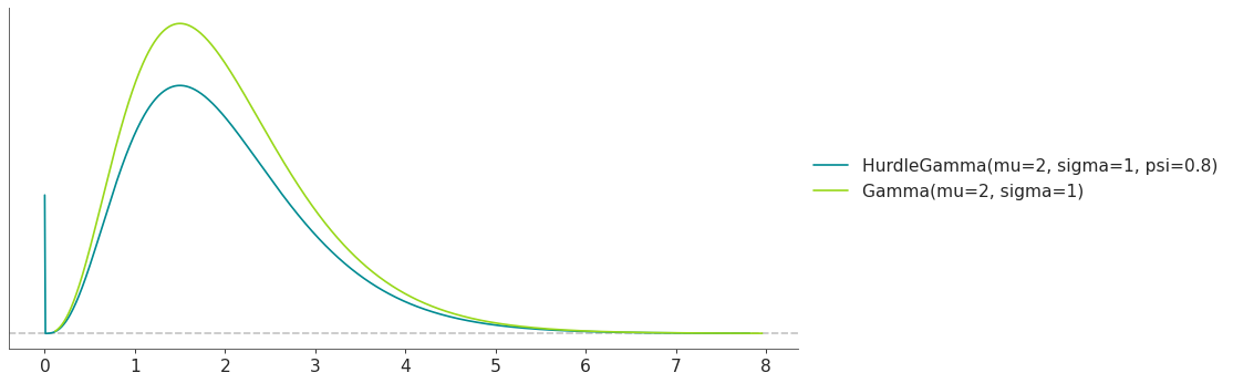
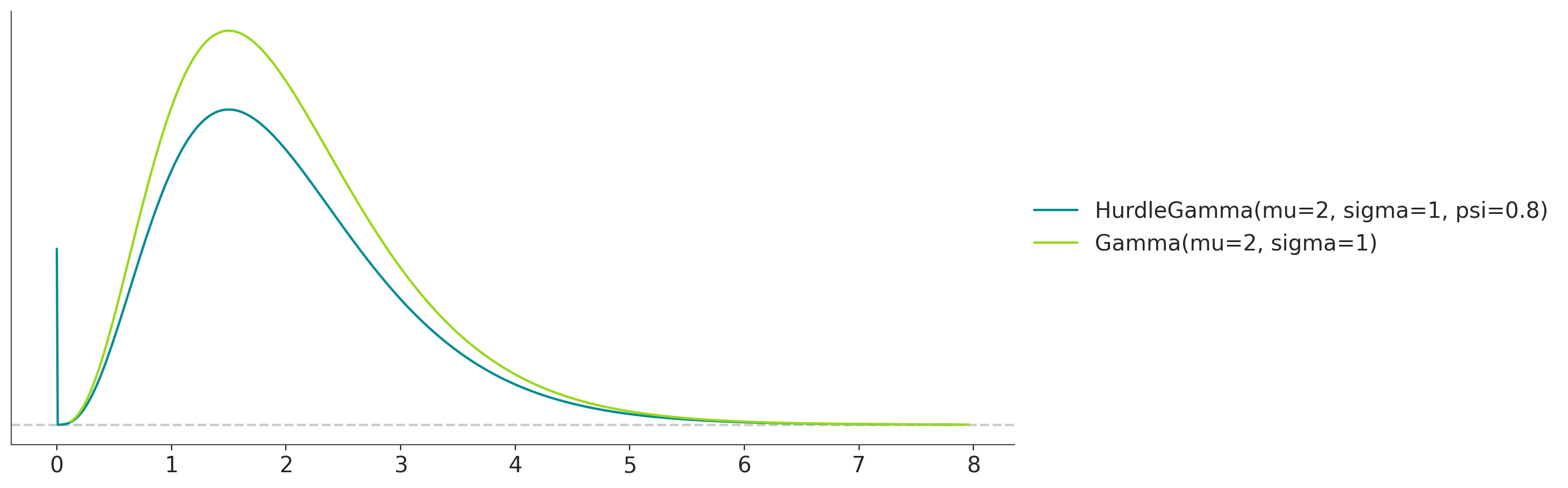
class preliz.distributions.mixture.Mixture(dists, weights=None)[source]#

Mixture distribution.

This is not a distribution per se, but a modifier of univariate distributions.

Given a series of base distributions with probability density mass/function ($p_i$). The pdf/pmf of a mixture distribution is:

\[f(x) = \sum_{i=1}^n \, w_i \, p_i(x)\]

(Source code, png, hires.png, pdf)

Parameters:

dists (List of Univariate PreliZ distributions) – Components of the mixture. They should be all discrete or all continuous.
weights (list of floats) – Weights must be larger or equal to 0 and their sum must be positive. If the weights do not sum up to 1, they will be normalized.

cdf(x)[source]#

Cumulative distribution function.

Parameters:: x (array_like) – Values on which to evaluate the cdf

entropy()[source]#: Entropy.

eti(mass=None, fmt='.2f')#

Equal-tailed interval containing mass.

Parameters:

mass (float) – Probability mass in the interval. Defaults to None,
used. (which results in the value of rcParams["stats.ci_prob"] being)
fmt (str) – fmt used to represent results using f-string fmt for floats. Default to “.2f” i.e. 2 digits after the decimal point. Use “none” for no format.

hdi(mass=None, fmt='.2f')#

Highest density interval containing mass.

Parameters:

mass (float) – Probability mass in the interval. Defaults to None,
used. (which results in the value of rcParams["stats.ci_prob"] being)
fmt (str) – fmt used to represent results using f-string fmt for floats. Default to “.2f” i.e. 2 digits after the decimal point. Use “none” for no format.

isf(x)#

Inverse survival function (inverse of sf).

Parameters:: x (array_like) – Values on which to evaluate the inverse of the sf

kurtosis()[source]#: Excess kurtosis.

lmoment1()#: L-moment1 (mean).

lmoment2()#: L-moment2 (l-scale).

lmoment3()#: L-moment3 (l-skewness). This the ratio of L-moment3 to L-moment2.

lmoment4()#: L-moment4 (l-kurtosis). This the ratio of L-moment4 to L-moment2.

lmoments(types='1234')#

Compute L-moments of the distribution.

Parameters:: types (str) – The type of moments to compute. Default is ‘1234’ where ‘1’ = L-moment1 (mean), ‘2’ = L-moment2 (l-scale), ‘3’ = L-moment3 (l-skewness), and ‘4’ = L-moment4 (l-kurtosis). To compute the standard deviation use ‘d’ Valid combinations are any subset of ‘1234’.

logcdf(x)#

Log cumulative distribution function.

Parameters:: x (array_like) – Values on which to evaluate the logcdf

logpdf(x)[source]#

Log probability density/mass function.

Parameters:: x (array_like) – Values on which to evaluate the logpdf

logsf(x)#

Log survival function log(1 - cdf).

Parameters:: x (array_like) – Values on which to evaluate the logsf

mean()[source]#: Mean.

median()[source]#: Median.

mode()#: Mode.

moments(types='mvsk')#

Compute moments of the distribution.

It can also return the standard deviation

Parameters:: types (str) – The type of moments to compute. Default is ‘mvsk’ where ‘m’ = mean, ‘v’ = variance, ‘s’ = skewness, and ‘k’ = kurtosis. To compute the standard deviation use ‘d’ Valid combinations are any subset of ‘mvdsk’.

pdf(x)[source]#

Probability density/mass function.

Parameters:: x (array_like) – Values on which to evaluate the pdf

plot_cdf(moments=None, pointinterval=False, interval=None, levels=None, support='restricted', legend='legend', figsize=None, ax=None, **kwargs)#

Plot the cumulative distribution function.

Parameters:

moments (str) – Compute moments. Use any combination of the strings m, d, v, s or k for the mean (μ), standard deviation (σ), variance (σ²), skew (γ) or kurtosis (κ) respectively. Other strings will be ignored. Defaults to None.
pointinterval (bool) – Whether to include a plot of the quantiles. Defaults to False. If True the default is to plot the median and two interquantiles ranges.
interval (str) – Type of interval. Available options are highest density interval “hdi” (default), equal tailed interval “eti” or intervals defined by arbitrary “quantiles”. Defaults to the value in rcParams[“stats.ci_kind”].
levels (list) – Mass of the intervals. For hdi or eti the number of elements should be 2 or 1. For quantiles the number of elements should be 5, 3, 1 or 0 (in this last case nothing will be plotted).
support (str:) – If full use the finite end-points to set the limits of the plot. For unbounded end-points or if restricted use the 0.001 and 0.999 quantiles to set the limits.
legend (str) – Whether to include a string with the distribution and its parameter as a "legend" a "title" or not include them None.
figsize (tuple) – Size of the figure
ax (matplotlib axes)
kwargs (keyword arguments) – Additional keyword arguments passed to matplotlib plot function. For example, color, alpha, linewidth, etc.

plot_interactive(kind='pdf', xy_lim='both', pointinterval=True, interval=None, levels=None, figsize=None)#

Interactive exploration of distributions parameters.

Parameters:

kind (str:) – Type of plot. Available options are pdf, cdf and ppf.
xy_lim (str or tuple) – Set the limits of the x-axis and/or y-axis. Defaults to “both”, the limits of both axis are fixed. Use “auto” for automatic rescaling of x-axis and y-axis. Or set them manually by passing a tuple of 4 elements, the first two for x-axis, the last two for y-axis. The tuple can have None.
pointinterval (bool) – Whether to include a plot of the quantiles. Defaults to False. If True the default is to plot the median and two interquantiles ranges.
interval (str) – Type of interval. Available options are highest density interval “hdi” (default), equal tailed interval “eti” or intervals defined by arbitrary “quantiles”. Defaults to the value in rcParams[“stats.ci_kind”].
levels (list) – Mass of the intervals. For hdi or eti the number of elements should be 2 or 1. For quantiles the number of elements should be 5, 3, 1 or 0 (in this last case nothing will be plotted).
figsize (tuple) – Size of the figure

plot_isf(moments=None, pointinterval=False, interval=None, levels=None, legend='legend', figsize=None, ax=None, **kwargs)#

Plot the inverse survival function.

Parameters:

moments (str) – Compute moments. Use any combination of the strings m, d, v, s or k for the mean (μ), standard deviation (σ), variance (σ²), skew (γ) or kurtosis (κ) respectively. Other strings will be ignored. Defaults to None.
pointinterval (bool) – Whether to include a plot of the quantiles. Defaults to False. If True the default is to plot the median and two interquantiles ranges.
interval (str) – Type of interval. Available options are highest density interval “hdi” (default), equal tailed interval “eti” or intervals defined by arbitrary “quantiles”. Defaults to the value in rcParams[“stats.ci_kind”].
levels (list) – Mass of the intervals. For hdi or eti the number of elements should be 2 or 1. For quantiles the number of elements should be 5, 3, 1 or 0 (in this last case nothing will be plotted).
legend (str) – Whether to include a string with the distribution and its parameter as a "legend" a "title" or not include them None.
figsize (tuple) – Size of the figure
ax (matplotlib axes)

plot_pdf(moments=None, pointinterval=False, interval=None, levels=None, support='restricted', baseline=True, legend='legend', figsize=None, ax=None, **kwargs)#

Plot the pdf (continuous) or pmf (discrete).

Parameters:

moments (str) – Compute moments. Use any combination of the strings m, d, v, s or k for the mean (μ), standard deviation (σ), variance (σ²), skew (γ) or kurtosis (κ) respectively. Other strings will be ignored. Defaults to None.
pointinterval (bool) – Whether to include a plot of the quantiles. Defaults to False. If True the default is to plot the median and two interquantiles ranges.
interval (str) – Type of interval. Available options are highest density interval “hdi” (default), equal tailed interval “eti” or intervals defined by arbitrary “quantiles”. Defaults to the value in rcParams[“stats.ci_kind”].
levels (list) – Mass of the intervals. For hdi or eti the number of elements should be 2 or 1. For quantiles the number of elements should be 5, 3, 1 or 0 (in this last case nothing will be plotted).
support (str:) – If full use the finite end-points to set the limits of the plot. For unbounded end-points or if restricted use the 0.001 and 0.999 quantiles to set the limits.
baseline (bool) – Whether to include a horizontal line at y=0.
legend (str) – Whether to include a string with the distribution and its parameter as a "legend" a "title" or not include them None.
figsize (tuple) – Size of the figure
ax (matplotlib axes)
kwargs (keyword arguments) – Additional keyword arguments passed to matplotlib plot function. For example, color, alpha, linewidth, etc.

plot_ppf(moments=None, pointinterval=False, interval=None, levels=None, legend='legend', figsize=None, ax=None, **kwargs)#

Plot the quantile function.

Parameters:

moments (str) – Compute moments. Use any combination of the strings m, d, v, s or k for the mean (μ), standard deviation (σ), variance (σ²), skew (γ) or kurtosis (κ) respectively. Other strings will be ignored. Defaults to None.
pointinterval (bool) – Whether to include a plot of the quantiles. Defaults to False. If True the default is to plot the median and two interquantiles ranges.
interval (str) – Type of interval. Available options are highest density interval “hdi” (default), equal tailed interval “eti” or intervals defined by arbitrary “quantiles”. Defaults to the value in rcParams[“stats.ci_kind”].
levels (list) – Mass of the intervals. For hdi or eti the number of elements should be 2 or 1. For quantiles the number of elements should be 5, 3, 1 or 0 (in this last case nothing will be plotted).
legend (str) – Whether to include a string with the distribution and its parameter as a "legend" a "title" or not include them None.
figsize (tuple) – Size of the figure
ax (matplotlib axes)

plot_sf(moments=None, pointinterval=False, interval=None, levels=None, support='restricted', legend='legend', figsize=None, ax=None, **kwargs)#

Plot the survival distribution function (1 - CDF).

Parameters:

moments (str) – Compute moments. Use any combination of the strings m, d, v, s or k for the mean (μ), standard deviation (σ), variance (σ²), skew (γ) or kurtosis (κ) respectively. Other strings will be ignored. Defaults to None.
pointinterval (bool) – Whether to include a plot of the quantiles. Defaults to False. If True the default is to plot the median and two interquantiles ranges.
interval (str) – Type of interval. Available options are highest density interval “hdi” (default), equal tailed interval “eti” or intervals defined by arbitrary “quantiles”. Defaults to the value in rcParams[“stats.ci_kind”].
levels (list) – Mass of the intervals. For hdi or eti the number of elements should be 2 or 1. For quantiles the number of elements should be 5, 3, 1 or 0 (in this last case nothing will be plotted).
support (str:) – If full use the finite end-points to set the limits of the plot. For unbounded end-points or if restricted use the 0.001 and 0.999 quantiles to set the limits.
legend (str) – Whether to include a string with the distribution and its parameter as a "legend" a "title" or not include them None.
figsize (tuple) – Size of the figure
ax (matplotlib axes)
kwargs (keyword arguments) – Additional keyword arguments passed to matplotlib plot function. For example, color, alpha, linewidth, etc.

ppf(q)[source]#

Percent point function (inverse of cdf).

Parameters:: x (array_like) – Values on which to evaluate the inverse of the cdf

rvs(size=None, random_state=None)[source]#

Random sample.

Parameters:

size (int or tuple of ints, optional) – Defining number of random variates. Defaults to 1.
random_state ({None, int, numpy.random.Generator, numpy.random.RandomState}) – Defaults to None

sf(x)#

Survival function (1 - cdf).

Parameters:: x (array_like) – Values on which to evaluate the sf

skewness()[source]#: Skewness.

std()[source]#: Standard deviation.

summary(mass=None, interval=None, fmt='.2f')#

Namedtuple with the mean, median, sd, and lower and upper bounds.

Parameters:

mass (float) – Probability mass for the equal-tailed interval. Defaults to None,
used. (which results in the value of rcParams["stats.ci_prob"] being)
interval (str or list-like) – Type of interval. Available options are highest density interval “hdi”, equal tailed interval “eti” or arbitrary interval defined by a list-like object with a pair of values. Defaults to the value in rcParams[“stats.ci_kind”].
fmt (str) – fmt used to represent results using f-string fmt for floats. Default to “.2f” i.e. 2 digits after the decimal point.

to_bambi(**kwargs)#

Convert the PreliZ distribution to a Bambi Prior.

kwargsPyMC distributions properties: kwargs are used to specify properties such as shape or dims

Return type:: Bambi Prior

to_pymc(name=None, **kwargs)#

Convert the PreliZ distribution to a PyMC distribution.

namestr: Name of PyMC distribution. Needed if inside Model context
kwargsPyMC distributions properties: kwargs are used to specify properties such as shape or dims

Return type:: PyMC distribution

var()[source]#: Variance.

xvals(support, n_points=None)#

Provide x values in the support of the distribution.

This is useful for example when plotting.

Parameters:

support (str) – Available options are “full” or “restricted”. If “full” the values will cover the entire support of the distribution if the boundary is finite, or the quantiles 0.0001 or 0.9999, if infinite. If “restricted” the values will cover the quantile 0.0001 to 0.9999.
n_points (int) – Number of values to return. Defaults to 1000 for continuous distributions and 200 for discrete ones. For discrete distributions the returned values may be fewer than n_points if the actual number of discrete values in the support of the distribution is smaller than n_points.

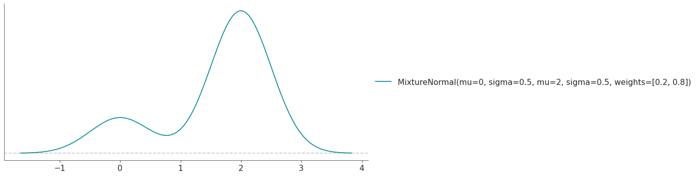
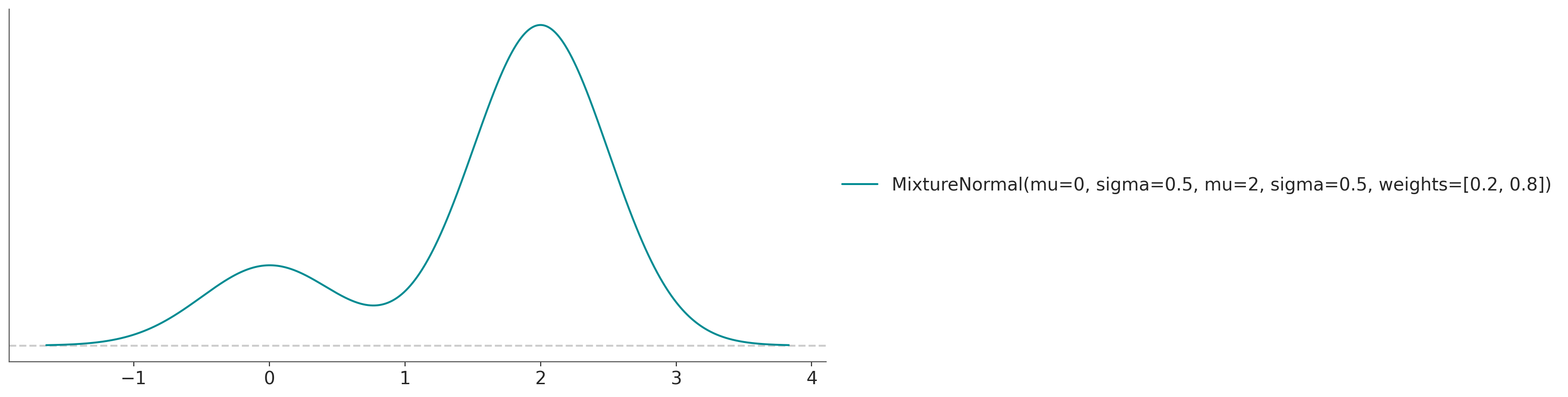
class preliz.distributions.truncated.Truncated(dist, lower=None, upper=None, **kwargs)[source]#

Truncated distribution.

This is not a distribution per se, but a modifier of univariate distributions.

Given a base distribution with cumulative distribution function (CDF) and probability density mass/function (PDF). The pdf of a Truncated distribution is:

\[\begin{split}\begin{cases} 0 & \text{for } x < \text{lower}, \\ \frac{\text{PDF}(x)}{\text{CDF}(upper) - \text{CDF}(lower)} & \text{for } \text{lower} <= x <= \text{upper}, \\ 0 & \text{for } x > \text{upper}, \end{cases}\end{split}\]

(Source code, png, hires.png, pdf)

Parameters:

dist (PreliZ distribution) – Univariate PreliZ distribution which will be truncated.
lower (float or int) – Lower (left) truncation point. Use np.inf for no truncation.
upper (float or int) – Upper (right) truncation point. Use np.inf for no truncation.

cdf(x)[source]#

Cumulative distribution function.

Parameters:: x (array_like) – Values on which to evaluate the cdf

entropy()[source]#: Entropy.

eti(mass=None, fmt='.2f')#

Equal-tailed interval containing mass.

Parameters:

mass (float) – Probability mass in the interval. Defaults to None,
used. (which results in the value of rcParams["stats.ci_prob"] being)
fmt (str) – fmt used to represent results using f-string fmt for floats. Default to “.2f” i.e. 2 digits after the decimal point. Use “none” for no format.

hdi(mass=None, fmt='.2f')#

Highest density interval containing mass.

Parameters:

mass (float) – Probability mass in the interval. Defaults to None,
used. (which results in the value of rcParams["stats.ci_prob"] being)
fmt (str) – fmt used to represent results using f-string fmt for floats. Default to “.2f” i.e. 2 digits after the decimal point. Use “none” for no format.

isf(x)#

Inverse survival function (inverse of sf).

Parameters:: x (array_like) – Values on which to evaluate the inverse of the sf

kurtosis()[source]#: Excess kurtosis.

lmoment1()#: L-moment1 (mean).

lmoment2()#: L-moment2 (l-scale).

lmoment3()#: L-moment3 (l-skewness). This the ratio of L-moment3 to L-moment2.

lmoment4()#: L-moment4 (l-kurtosis). This the ratio of L-moment4 to L-moment2.

lmoments(types='1234')#

Compute L-moments of the distribution.

Parameters:: types (str) – The type of moments to compute. Default is ‘1234’ where ‘1’ = L-moment1 (mean), ‘2’ = L-moment2 (l-scale), ‘3’ = L-moment3 (l-skewness), and ‘4’ = L-moment4 (l-kurtosis). To compute the standard deviation use ‘d’ Valid combinations are any subset of ‘1234’.

logcdf(x)#

Log cumulative distribution function.

Parameters:: x (array_like) – Values on which to evaluate the logcdf

logpdf(x)[source]#

Log probability density/mass function.

Parameters:: x (array_like) – Values on which to evaluate the logpdf

logsf(x)#

Log survival function log(1 - cdf).

Parameters:: x (array_like) – Values on which to evaluate the logsf

mean()[source]#: Mean.

median()[source]#: Median.

mode()[source]#: Mode.

moments(types='mvsk')#

Compute moments of the distribution.

It can also return the standard deviation

Parameters:: types (str) – The type of moments to compute. Default is ‘mvsk’ where ‘m’ = mean, ‘v’ = variance, ‘s’ = skewness, and ‘k’ = kurtosis. To compute the standard deviation use ‘d’ Valid combinations are any subset of ‘mvdsk’.

pdf(x)[source]#

Probability density/mass function.

Parameters:: x (array_like) – Values on which to evaluate the pdf

plot_cdf(moments=None, pointinterval=False, interval=None, levels=None, support='restricted', legend='legend', figsize=None, ax=None, **kwargs)#

Plot the cumulative distribution function.

Parameters:

moments (str) – Compute moments. Use any combination of the strings m, d, v, s or k for the mean (μ), standard deviation (σ), variance (σ²), skew (γ) or kurtosis (κ) respectively. Other strings will be ignored. Defaults to None.
pointinterval (bool) – Whether to include a plot of the quantiles. Defaults to False. If True the default is to plot the median and two interquantiles ranges.
interval (str) – Type of interval. Available options are highest density interval “hdi” (default), equal tailed interval “eti” or intervals defined by arbitrary “quantiles”. Defaults to the value in rcParams[“stats.ci_kind”].
levels (list) – Mass of the intervals. For hdi or eti the number of elements should be 2 or 1. For quantiles the number of elements should be 5, 3, 1 or 0 (in this last case nothing will be plotted).
support (str:) – If full use the finite end-points to set the limits of the plot. For unbounded end-points or if restricted use the 0.001 and 0.999 quantiles to set the limits.
legend (str) – Whether to include a string with the distribution and its parameter as a "legend" a "title" or not include them None.
figsize (tuple) – Size of the figure
ax (matplotlib axes)
kwargs (keyword arguments) – Additional keyword arguments passed to matplotlib plot function. For example, color, alpha, linewidth, etc.

plot_interactive(kind='pdf', xy_lim='both', pointinterval=True, interval=None, levels=None, figsize=None)#

Interactive exploration of distributions parameters.

Parameters:

kind (str:) – Type of plot. Available options are pdf, cdf and ppf.
xy_lim (str or tuple) – Set the limits of the x-axis and/or y-axis. Defaults to “both”, the limits of both axis are fixed. Use “auto” for automatic rescaling of x-axis and y-axis. Or set them manually by passing a tuple of 4 elements, the first two for x-axis, the last two for y-axis. The tuple can have None.
pointinterval (bool) – Whether to include a plot of the quantiles. Defaults to False. If True the default is to plot the median and two interquantiles ranges.
interval (str) – Type of interval. Available options are highest density interval “hdi” (default), equal tailed interval “eti” or intervals defined by arbitrary “quantiles”. Defaults to the value in rcParams[“stats.ci_kind”].
levels (list) – Mass of the intervals. For hdi or eti the number of elements should be 2 or 1. For quantiles the number of elements should be 5, 3, 1 or 0 (in this last case nothing will be plotted).
figsize (tuple) – Size of the figure

plot_isf(moments=None, pointinterval=False, interval=None, levels=None, legend='legend', figsize=None, ax=None, **kwargs)#

Plot the inverse survival function.

Parameters:

moments (str) – Compute moments. Use any combination of the strings m, d, v, s or k for the mean (μ), standard deviation (σ), variance (σ²), skew (γ) or kurtosis (κ) respectively. Other strings will be ignored. Defaults to None.
pointinterval (bool) – Whether to include a plot of the quantiles. Defaults to False. If True the default is to plot the median and two interquantiles ranges.
interval (str) – Type of interval. Available options are highest density interval “hdi” (default), equal tailed interval “eti” or intervals defined by arbitrary “quantiles”. Defaults to the value in rcParams[“stats.ci_kind”].
levels (list) – Mass of the intervals. For hdi or eti the number of elements should be 2 or 1. For quantiles the number of elements should be 5, 3, 1 or 0 (in this last case nothing will be plotted).
legend (str) – Whether to include a string with the distribution and its parameter as a "legend" a "title" or not include them None.
figsize (tuple) – Size of the figure
ax (matplotlib axes)

plot_pdf(moments=None, pointinterval=False, interval=None, levels=None, support='restricted', baseline=True, legend='legend', figsize=None, ax=None, **kwargs)#

Plot the pdf (continuous) or pmf (discrete).

Parameters:

moments (str) – Compute moments. Use any combination of the strings m, d, v, s or k for the mean (μ), standard deviation (σ), variance (σ²), skew (γ) or kurtosis (κ) respectively. Other strings will be ignored. Defaults to None.
pointinterval (bool) – Whether to include a plot of the quantiles. Defaults to False. If True the default is to plot the median and two interquantiles ranges.
interval (str) – Type of interval. Available options are highest density interval “hdi” (default), equal tailed interval “eti” or intervals defined by arbitrary “quantiles”. Defaults to the value in rcParams[“stats.ci_kind”].
levels (list) – Mass of the intervals. For hdi or eti the number of elements should be 2 or 1. For quantiles the number of elements should be 5, 3, 1 or 0 (in this last case nothing will be plotted).
support (str:) – If full use the finite end-points to set the limits of the plot. For unbounded end-points or if restricted use the 0.001 and 0.999 quantiles to set the limits.
baseline (bool) – Whether to include a horizontal line at y=0.
legend (str) – Whether to include a string with the distribution and its parameter as a "legend" a "title" or not include them None.
figsize (tuple) – Size of the figure
ax (matplotlib axes)
kwargs (keyword arguments) – Additional keyword arguments passed to matplotlib plot function. For example, color, alpha, linewidth, etc.

plot_ppf(moments=None, pointinterval=False, interval=None, levels=None, legend='legend', figsize=None, ax=None, **kwargs)#

Plot the quantile function.

Parameters:

moments (str) – Compute moments. Use any combination of the strings m, d, v, s or k for the mean (μ), standard deviation (σ), variance (σ²), skew (γ) or kurtosis (κ) respectively. Other strings will be ignored. Defaults to None.
pointinterval (bool) – Whether to include a plot of the quantiles. Defaults to False. If True the default is to plot the median and two interquantiles ranges.
interval (str) – Type of interval. Available options are highest density interval “hdi” (default), equal tailed interval “eti” or intervals defined by arbitrary “quantiles”. Defaults to the value in rcParams[“stats.ci_kind”].
levels (list) – Mass of the intervals. For hdi or eti the number of elements should be 2 or 1. For quantiles the number of elements should be 5, 3, 1 or 0 (in this last case nothing will be plotted).
legend (str) – Whether to include a string with the distribution and its parameter as a "legend" a "title" or not include them None.
figsize (tuple) – Size of the figure
ax (matplotlib axes)

plot_sf(moments=None, pointinterval=False, interval=None, levels=None, support='restricted', legend='legend', figsize=None, ax=None, **kwargs)#

Plot the survival distribution function (1 - CDF).

Parameters:

moments (str) – Compute moments. Use any combination of the strings m, d, v, s or k for the mean (μ), standard deviation (σ), variance (σ²), skew (γ) or kurtosis (κ) respectively. Other strings will be ignored. Defaults to None.
pointinterval (bool) – Whether to include a plot of the quantiles. Defaults to False. If True the default is to plot the median and two interquantiles ranges.
interval (str) – Type of interval. Available options are highest density interval “hdi” (default), equal tailed interval “eti” or intervals defined by arbitrary “quantiles”. Defaults to the value in rcParams[“stats.ci_kind”].
levels (list) – Mass of the intervals. For hdi or eti the number of elements should be 2 or 1. For quantiles the number of elements should be 5, 3, 1 or 0 (in this last case nothing will be plotted).
support (str:) – If full use the finite end-points to set the limits of the plot. For unbounded end-points or if restricted use the 0.001 and 0.999 quantiles to set the limits.
legend (str) – Whether to include a string with the distribution and its parameter as a "legend" a "title" or not include them None.
figsize (tuple) – Size of the figure
ax (matplotlib axes)
kwargs (keyword arguments) – Additional keyword arguments passed to matplotlib plot function. For example, color, alpha, linewidth, etc.

ppf(q)[source]#

Percent point function (inverse of cdf).

Parameters:: x (array_like) – Values on which to evaluate the inverse of the cdf

rvs(size=None, random_state=None)[source]#

Random sample.

Parameters:

size (int or tuple of ints, optional) – Defining number of random variates. Defaults to 1.
random_state ({None, int, numpy.random.Generator, numpy.random.RandomState}) – Defaults to None

sf(x)#

Survival function (1 - cdf).

Parameters:: x (array_like) – Values on which to evaluate the sf

skewness()[source]#: Skewness.

std()[source]#: Standard deviation.

summary(mass=None, interval=None, fmt='.2f')#

Namedtuple with the mean, median, sd, and lower and upper bounds.

Parameters:

mass (float) – Probability mass for the equal-tailed interval. Defaults to None,
used. (which results in the value of rcParams["stats.ci_prob"] being)
interval (str or list-like) – Type of interval. Available options are highest density interval “hdi”, equal tailed interval “eti” or arbitrary interval defined by a list-like object with a pair of values. Defaults to the value in rcParams[“stats.ci_kind”].
fmt (str) – fmt used to represent results using f-string fmt for floats. Default to “.2f” i.e. 2 digits after the decimal point.

to_bambi(**kwargs)#

Convert the PreliZ distribution to a Bambi Prior.

kwargsPyMC distributions properties: kwargs are used to specify properties such as shape or dims

Return type:: Bambi Prior

to_pymc(name=None, **kwargs)#

Convert the PreliZ distribution to a PyMC distribution.

namestr: Name of PyMC distribution. Needed if inside Model context
kwargsPyMC distributions properties: kwargs are used to specify properties such as shape or dims

Return type:: PyMC distribution

var()[source]#: Variance.

xvals(support, n_points=None)#

Provide x values in the support of the distribution.

This is useful for example when plotting.

Parameters:

support (str) – Available options are “full” or “restricted”. If “full” the values will cover the entire support of the distribution if the boundary is finite, or the quantiles 0.0001 or 0.9999, if infinite. If “restricted” the values will cover the quantile 0.0001 to 0.9999.
n_points (int) – Number of values to return. Defaults to 1000 for continuous distributions and 200 for discrete ones. For discrete distributions the returned values may be fewer than n_points if the actual number of discrete values in the support of the distribution is smaller than n_points.

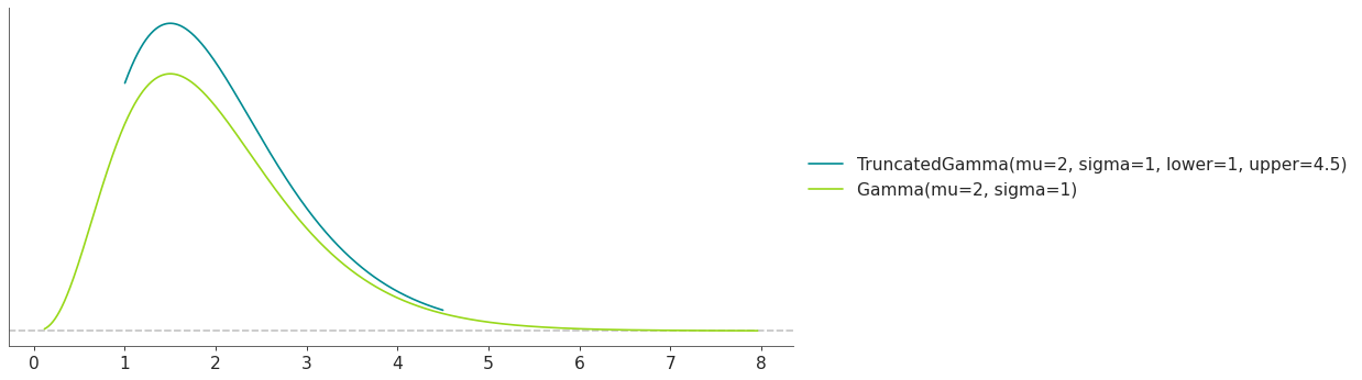
`preliz.distributions`#

preliz.distributions.plot.plot(dist, kind='pdf', moments=None, marginals=True, pointinterval=False, interval=None, levels=None, support='restricted', baseline=True, legend='legend', figsize=None, ax=None, **kwargs)[source]#

Plot distribution functions, including pdf, cdf, ppf, sf and isf.

Parameters:

kind (str) – Specify which distribution function to plot. Defaults to pdf, i.e. the probability density function for continuos distributions or probability mass function for discrete distributions. Others possible values are: * cdf cumulative distribution function * ppf percent point function, also know as inverse of the cdf * sf survival function (1-cdf) * isf inverse survival function
moments (str) – Compute moments. Use any combination of the strings m, d, v, s or k for the mean (μ), standard deviation (σ), variance (σ²), skew (γ) or kurtosis (κ) respectively. Other strings will be ignored. Defaults to None. Ignored for multivariate distributions.
marginals (bool) – Whether to plot the marginals of the distribution. Only used when plotting multivariate distributions and kind="pdf". Defaults to True. If False the joint distribution will be plotted when possible.
pointinterval (bool) – Whether to include a plot of the quantiles. Defaults to False. If True the default is to plot the median and two interquantiles ranges.
interval (str) – Type of interval. Available options are highest density interval “hdi” (default), equal tailed interval “eti” or intervals defined by arbitrary “quantiles”. Defaults to the value in rcParams[“stats.ci_kind”].
levels (list) – Mass of the intervals. For hdi or eti the number of elements should be 2 or 1. For quantiles the number of elements should be 5, 3, 1 or 0 (in this last case nothing will be plotted).
support (str:) – If full use the finite end-points to set the limits of the plot. For unbounded end-points or if restricted use the 0.001 and 0.999 quantiles to set the limits. Ignored when kind="ppf", kind="isf".
baseline (bool) – Whether to include a horizontal line at y=0. Only used when kind="pdf", ignored otherwise.
legend (str) – Whether to include a string with the distribution and its parameter as a "legend" a "title" or not include them None.
figsize (tuple) – Size of the figure
ax (matplotlib axes)
kwargs (keyword arguments) – Additional keyword arguments passed to matplotlib plot function. For example, color, alpha, linewidth, etc.

Support	\(x \in \mathbb{R}\)
Mean	\(\mu-\frac{\\\kappa-1/\kappa}b\)
Variance	\(\frac{1+\kappa^{4}}{b^2\kappa^2 }\)

Support	\(x \in (0, 1)\)
Mean	\(\dfrac{\alpha}{\alpha + \beta}\)
Variance	\(\dfrac{\alpha \beta}{(\alpha+\beta)^2(\alpha+\beta+1)}\)

Support	\(x \in (lower, upper)\)
Mean	\(\dfrac{\alpha}{\alpha + \beta} (upper-lower) + lower\)
Variance	\(\dfrac{\alpha \beta}{(\alpha+\beta)^2(\alpha+\beta+1)} (upper-lower)\)

Support	\(x \in [0, \infty)\)
Mean	\(\dfrac{1}{\lambda}\)
Variance	\(\dfrac{1}{\lambda^2}\)

Support	\(x \in (0, \infty)\)
Mean	\(\dfrac{\alpha}{\beta}\)
Variance	\(\dfrac{\alpha}{\beta^2}\)

Support	\(x \in (-\infty, \infty)\)
Mean	\(\mu + \sigma\left(\gamma + \log 2\right)\), where \(\gamma\) is the Euler-Mascheroni constant
Variance	\(\frac{\pi^{2}}{2}\sigma^{2}\)

Support	\(x \in [m, \infty)\)
Mean	\(\dfrac{\alpha m}{\alpha - 1}\) for \(\alpha \ge 1\)
Variance	\(\dfrac{m^2 \alpha}{(\alpha - 1)^2 (\alpha - 2)}\) for \(\alpha > 2\)

Support	\(x \in [lower, upper]\)
Mean	\(\dfrac{lower + upper + c}{3}\)
Variance	\(\dfrac{upper^2 + lower^2 +c^2 - lowerupper - lowerc - upper*c}{18}\)

Support	\(x \in [a, b]\)
Mean	\(\mu +{\frac {\phi (\alpha )-\phi (\beta )}{Z}}\sigma\)
Variance	\[\sigma ^{2}\left[1+{\frac {\alpha \phi (\alpha )-\beta \phi (\beta )}{Z}}- \left({\frac {\phi (\alpha )-\phi (\beta )}{Z}}\right)^{2}\right]\]

Support	\(x \in [-\pi, \pi]\)
Mean	\(\mu\)
Variance	\(1-\frac{I_1(\kappa)}{I_0(\kappa)}\)

Support	\(x \in \{0, 1, \ldots, n\}\)
Mean	\(n \dfrac{\alpha}{\alpha + \beta}\)
Variance	\(\dfrac{n \alpha \beta (\alpha+\beta+n)}{(\alpha+\beta)^2 (\alpha+\beta+1)}\)

Support	\(x \in {lower, lower + 1, \ldots, upper}\)
Mean	\(\dfrac{lower + upper}{2}\)
Variance	\(\dfrac{(upper - lower + 1)^2 - 1}{12}\)

Support	\(x \in \mathbb{N}_0\)
Mean	\(\mu = \sum_{x = 1}^{\infty} q^{x^{\beta}}\)
Variance	\(2 \sum_{x = 1}^{\infty} x q^{x^{\beta}} - \mu - \mu^2\)

Support	\(x \in \mathbb{N}_{>0}\)
Mean	\(\dfrac{1}{p}\)
Variance	\(\dfrac{1 - p}{p^2}\)

Support	\(x \in \left[\max(0, n - N + k), \min(k, n)\right]\)
Mean	\(\dfrac{nk}{N}\)
Variance	\(\dfrac{(N-n)nk(N-k)}{(N-1)N^2}\)

Support	\(x_i \in (0, 1)\) for \(i \in \{1, \ldots, K\}\) such that \(\sum x_i = 1\)
Mean	\(\dfrac{a_i}{\sum a_i}\)
Variance	\(\dfrac{a_i - \sum a_0}{a_0^2 (a_0 + 1)}\) where \(a_0 = \sum a_i\)

Distributions#

preliz.distributions.continuous#

preliz.distributions.discrete#

preliz.distributions.continuous_multivariate#

preliz.distributions#

preliz.distributions#

`preliz.distributions.continuous`#

`preliz.distributions.discrete`#

`preliz.distributions.continuous_multivariate`#

`preliz.distributions`#

`preliz.distributions`#