Unidimensional#

`preliz.unidimensional`#

class preliz.unidimensional.QuartileInt(q1=1, q2=2, q3=3, dist_names=None, figsize=None)[source]#

Prior elicitation for 1D distributions from quartiles (See Morris et al.[1]).

Parameters:

q1 (float) – First quartile, i.e 0.25 of the mass is below this point.
q2 (float) – Second quartile, i.e 0.50 of the mass is below this point. This is also know as the median.
q3 (float) – Third quartile, i.e 0.75 of the mass is below this point.
dist_names (list) – List of distributions names to be used in the elicitation. If None, almost all 1D distributions available in PreliZ will be used. Some distributions like Uniform or Cauchy are omitted by default.
figsize (Optional[Tuple[int, int]]) – Figure size. If None it will be defined automatically.

Note

Use the params text box to parametrize distributions, for instance write BetaScaled(lower=-1, upper=10) to specify the upper and lower bounds of BetaScaled distribution. To parametrize more that one distribution use commas for example StudentT(nu=3), TruncatedNormal(lower=-2, upper=inf)

References

class preliz.unidimensional.Roulette(x_min=0, x_max=10, nrows=10, ncols=11, dist_names=None, params=None, figsize=None)[source]#

Prior elicitation for 1D distribution using the roulette method (See Morris et al.[1]).

Draw 1D distributions using a grid as input.

Parameters:

x_min (Optional[float]) – Minimum value for the domain of the grid and fitted distribution.
x_max (Optional[float]) – Maximum value for the domain of the grid and fitted distribution.
nrows (Optional[int]) – Number of rows for the grid. Defaults to 10.
ncols (Optional[int]) – Number of columns for the grid. Defaults to 11.
dist_names (list) – List of distribution names to be used in the elicitation. Defaults to None. The pre-selected distributions are [“Normal”, “BetaScaled”, “Gamma”, “LogNormal”, “StudentT”], but almost all 1D PreliZ’s distributions are available to be selected from the menu with some exceptions like Uniform or Cauchy.
params (Optional[str]) – Extra parameters to be passed to the distributions. The format is a string with the PreliZ’s distribution name followed by the argument to fix. For example: “TruncatedNormal(lower=0), StudentT(nu=8)”. If you use the params text area, quotation marks are not necessary.
figsize (Optional[Tuple[int, int]]) – Figure size. If None, it will be defined automatically.

Returns:

The object has many attributes, but the most important are: - dist: The fitted distribution. - inputs: A tuple with the x values, the empirical pdf, the total chips, the x_min, the x_max, the number of rows, and the number of columns.

Return type:

Roulette object

preliz.unidimensional.combine(distributions, weights=None, dist_names=None, sample_size=10000, rng=0, plot=1, plot_kwargs=None, ax=None)[source]#

Combine a set of distributions into a single one.

Fit a weighted sample from distributions into the distributions listed in ``dist_names`. The fit is done using maximum likelihood estimation, and the best match is plotted. Notice that the result is NOT a Mixture distribution, but a single distribution that best fits the weighted sample.

Parameters:

distributions (List of PreliZ distributions) – These are the distributions that we want to combine. Typically, these have been elicited from different individuals or instances.
weights (array-like, optional) – Weights for each distribution. Defaults to None, i.e. equal weights. The sum of the weights must be equal to 1, otherwise it will be normalized.
dist_names (list) – List of distributions to fit the weighted sample. Defaults to ["Normal", "Gamma", "LogNormal", "StudentT"].
sample_size (int) – Number of total samples to generate for the fit.
rng (int or numpy.random.Generator, optional) – Random number generator or seed. Defaults to 0.
plot (int) – Number of distributions to plots. Defaults to 1 (i.e. plot the best match) If larger than the number of passed distributions it will plot all of them. Use 0 or False to disable plotting.
plot_kwargs (dict) – Dictionary passed to the method plot_pdf().
ax (matplotlib axes)

Returns:

fitted_distributions (list of PreliZ distributions.) – The distributions that best fit the weighted sample. Sorted from best to worst match.
axes (matplotlib axes)

preliz.unidimensional.combine_roulette(responses, weights=None, dist_names=None, params=None)[source]#

Combine multiple elicited distributions into a single distribution.

Parameters:

responses (list of tuples) – Typically, each tuple comes from the .inputs attribute of a Roulette object and represents a single elicited distribution.
weights (array-like, optional) – Weights for each elicited distribution. Defaults to None, i.e. equal weights. The sum of the weights must be equal to 1, otherwise it will be normalized.
dist_names (list) – List of distributions names to be used in the elicitation. Defaults to [“Normal”, “BetaScaled”, “Gamma”, “LogNormal”, “StudentT”].
params (str, optional) – Extra parameters to be passed to the distributions. The format is a string with the PreliZ’s distribution name followed by the argument to fix. For example: “TruncatedNormal(lower=0), StudentT(nu=8)”.

Return type:

PreliZ distribution

preliz.unidimensional.match_moments(from_dist, to_dist, moments='mv', plot=None, plot_kwargs=None, ax=None)[source]#

Find the distribution to_dist that matches the moments of from_dist.

Parameters:

from_dist (PreliZ or PyMC distribution or array-like) – Instance of a fully parametrized PreliZ distribution or array-like data. We will take the moments from this distribution or data.
to_dist (PreliZ distribution or PyMC distribution) – Instance of a distribution to be fitted to match the moments of from_dist. If a PreliZ distribution then it can have some parameters fixed. PreliZ distributions are updated inplace.
moments (str) – The type of moments to compute. Default is ‘mv’ (mean and variance). Valid combinations are any subset of ‘mvdsk’, where ‘m’ = mean, ‘v’ = variance, ‘s’ = skewness, and ‘k’ = kurtosis. ‘d’ = standard deviation is also valid.
plot (bool) – Whether to plot the distributions. Defaults to None, which results in the value of rcParams[“plots.show_plot”] being used.
plot_kwargs (dict) – Dictionary passed to the method plot_pdf() of from_dist and to_dist.
ax (matplotlib axes)

Returns:

dict (PreliZ distribution)
axes (matplotlib axes (only if plot=True))

Notes

After calling this function the attribute opt of the distribution will be updated with the OptimizeResult object from the optimization step.

See also

match_quantiles: Match the distribution to the specified quantiles.

Examples

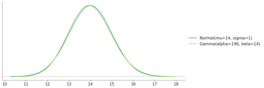
Moment matching between a known Normal and a Gamma distribution:

>>> import preliz as pz
>>> pz.style.use('preliz-doc')
>>> pz.match_moments(pz.Normal(14, 1), pz.Gamma())

(Source code, png, hires.png, pdf)

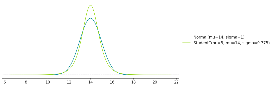
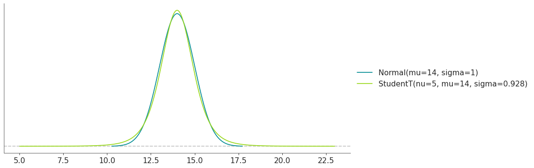
Moment matching between a known Normal and a StudentT distribution with nu fixed to 5:

>>> import preliz as pz
>>> pz.style.use('preliz-doc')
>>> pz.match_moments(pz.Normal(14, 1), pz.StudentT(nu=5))

(Source code, png, hires.png, pdf)

preliz.unidimensional.match_quantiles(from_dist, to_dist, quantiles=None, plot=None, plot_kwargs=None, ax=None)[source]#

Find the distribution to_dist that matches the moments of from_dist.

Parameters:

from_dist (PreliZ or PyMC distribution or array-like) – Instance of a fully parametrized PreliZ distribution or an array-like object. We will take the quantiles from this distribution or array.
to_dist (PreliZ distribution or PyMC distribution) – Instance of a distribution to be fitted to match the quantiles of from_dist. If a PreliZ distribution then it can have some parameters fixed. PreliZ distributions are updated inplace.
quantiles (array-like, optional) – Quantiles to match. Default is [0.25, 0.5, 0.75].
plot (bool) – Whether to plot the distributions. Defaults to None, which results in the value of rcParams[“plots.show_plot”] being used.
plot_kwargs (dict) – Dictionary passed to the method plot_pdf() of from_dist and to_dist.
ax (matplotlib axes)

Returns:

dict (PreliZ distribution)
axes (matplotlib axes (only if plot=True))

Notes

After calling this function the attribute opt of the distribution will be updated with the OptimizeResult object from the optimization step.

See also

match_moments: Match the distribution to the specified moments.

Examples

Moment matching between a known Normal and a Gamma distribution:

>>> import preliz as pz
>>> pz.style.use('preliz-doc')
>>> pz.match_quantiles(pz.Normal(14, 1), pz.Gamma())

(Source code, png, hires.png, pdf)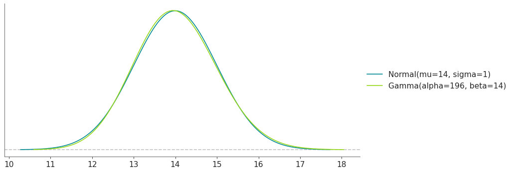

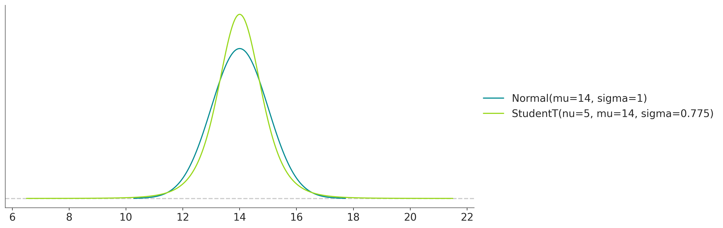
Moment matching between a known Normal and a StudentT distribution with nu fixed to 5:

>>> import preliz as pz
>>> pz.style.use('preliz-doc')
>>> pz.match_quantiles(pz.Normal(14, 1), pz.StudentT(nu=5))

(Source code, png, hires.png, pdf)

preliz.unidimensional.maxent(distribution=None, lower=-1, upper=1, mass=None, fixed_stat=None, fixed_params=None, plot=None, plot_kwargs=None, ax=None)[source]#

Find the maximum entropy distribution that satisfies the constraints.

Find the maximum entropy distribution with mass in the interval defined by the lower and upper end-points.

Parameters:

name (PreliZ or PyMC distribution) – PreliZ distribution are updated inplace, while PyMC distributions are converted to PreliZ distributions. Distributions can be partially initialized, i.e. some parameters can be fixed while others are left free to be estimated. For PreliZ distributions, set the parameters you want to fix and don’t set the rest. As an alternative fixed_params can be used. For PyMC distributions, set the parameters to np.nan, and use fixed_params in case you want to fix any of them.
lower (float) – Lower end-point
upper (float) – Upper end-point
mass (float) – Probability mass between lower and upper bounds. Defaults to None, which results in the value of rcParams[“stats.ci_prob”] being used.
fixed_stat (tuple) – Summary statistic to fix. The first element should be a name and the second a numerical value. Valid names are: “mean”, “mode”, “median”, “var”, “std”, “skewness”, “kurtosis”. Defaults to None.
fixed_params (dict) – Dictionary with parameter names as keys and the values to fix them to as values. If using a PreliZ distribution, parameters can also be fixed by setting them when initializing the distribution. Defaults to None.
plot (bool) – Whether to plot the distribution, and lower and upper bounds. Defaults to None, which results in the value of rcParams[“plots.show_plot”] being used.
plot_kwargs (dict) – Dictionary passed to the method plot_pdf() of distribution.
ax (matplotlib axes)

Returns:

dict (PreliZ distribution)
axes (matplotlib axes (only if plot=True))

Notes

After calling this function the attribute opt of the distribution will be updated with the OptimizeResult object from the optimization step.

See also

quartile: Find the distribution with the specified quartiles.

Examples

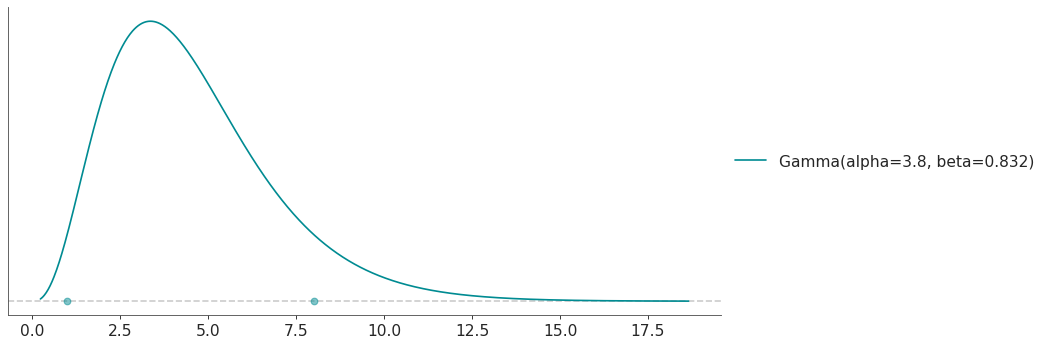
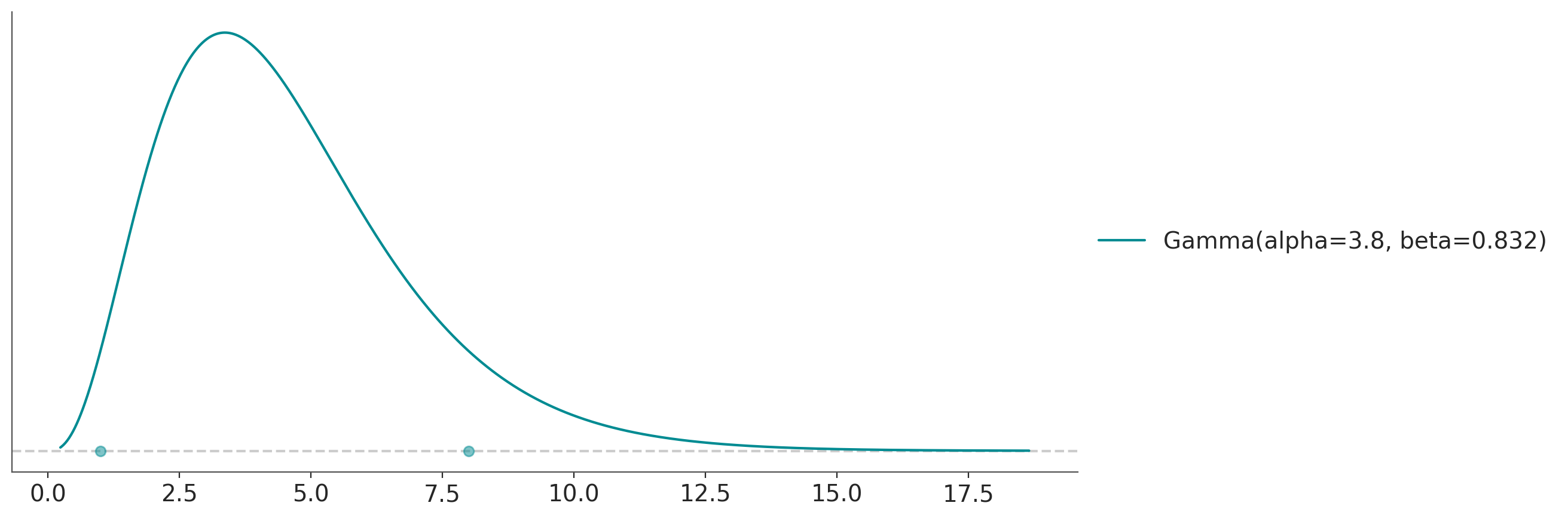
Calculate the maxent Gamma distribution with 90 % of the mass between 1 and 8:

>>> import preliz as pz
>>> pz.style.use('preliz-doc')
>>> pz.maxent(pz.Gamma(), 1, 8, 0.9)

(Source code, png, hires.png, pdf)

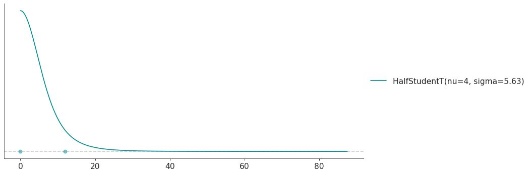
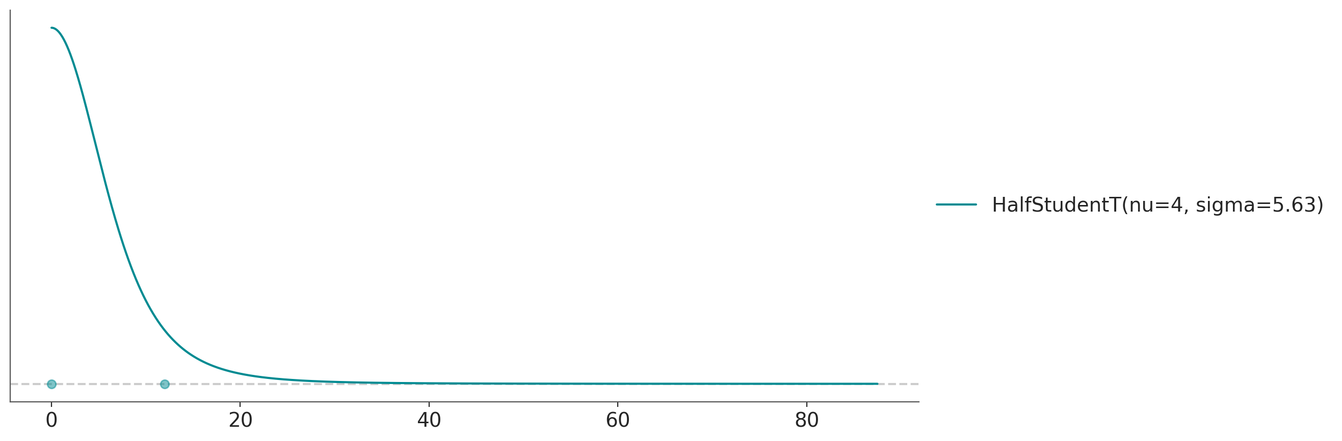
Calculate the maxent HalfStudentT T distribution with 90 % of the mass between 0 and 12 and a value of nu=4:

>>> import preliz as pz
>>> pz.style.use('preliz-doc')
>>> pz.maxent(pz.HalfStudentT(nu=4), 0, 12, 0.9)

(Source code, png, hires.png, pdf)

preliz.unidimensional.mle(distributions, sample, plot=1, plot_kwargs=None, ax=None)[source]#

Find the maximum likelihood distribution given a list of distributions and one sample.

AIC with a correction for small sample sizes is used to compare the fits. (See Burnham and Anderson[2])

Parameters:

distributions (list of PreliZ (or PyMC) distributions) – Instance of a distribution. Notice that the distributions will be updated inplace. If the distribution is from PyMC, it will be converted to a PreliZ distribution, use .to_pymc() to convert it back to PyMC. All parameters will be estimated from the data, no parameter can be fixed. For PreliZ distributions, pass uninitialized distributions. For some PyMC distributions, you may need to pass np.nan for parameters.
sample (list or 1D array-like) – Data used to estimate the distribution parameters.
plot (int) – Number of distributions to plots. Defaults to 1 (i.e. plot the best match) If larger than the number of passed distributions it will plot all of them. Use 0 or False to disable plotting. If you want to disable plotting globally you can also set rcParams["plots.show_plot"] = False.
plot_kwargs (dict) – Dictionary passed to the method plot_pdf() of distribution.
ax (matplotlib axes)

Returns:

idx (array with the indexes to sort distributions from best to worst match)
axes (matplotlib axes)

Examples

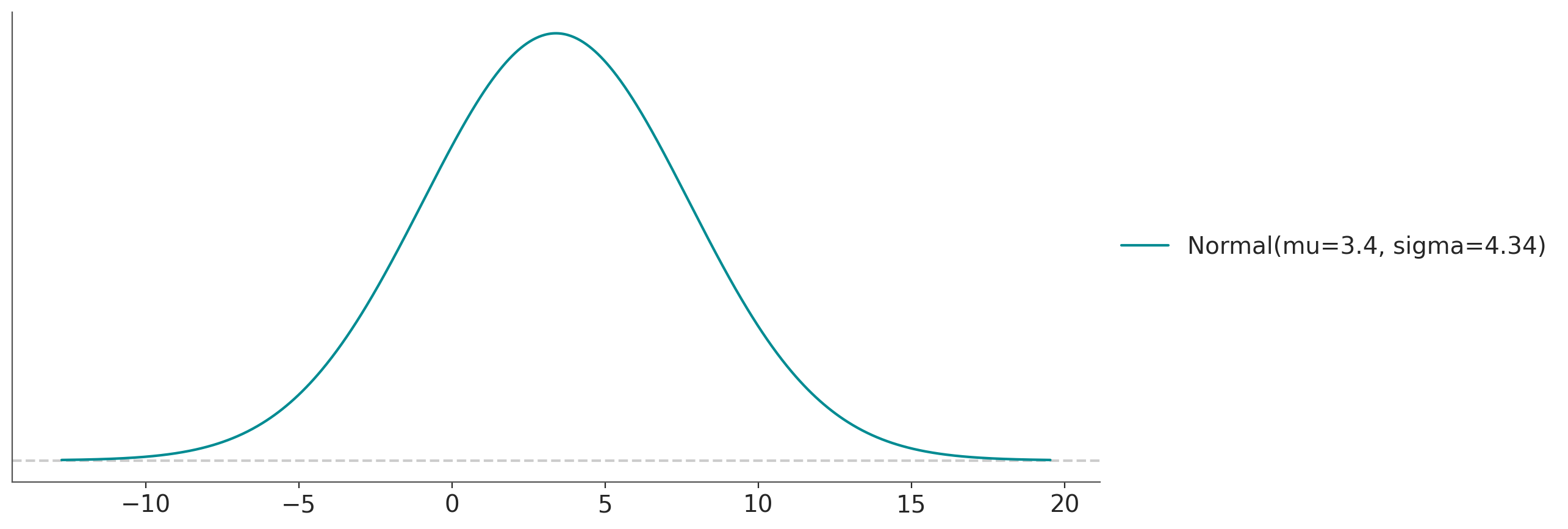
Fit a Normal and a Gamma distribution to data sampled from a Moyal distribution. In “real life” instead of a sample from a known distribution you would have some observed data.

>>> import preliz as pz
>>> pz.style.use('preliz-doc')
>>> sample = pz.Moyal(1, 2).rvs(1000)  # some random data
>>> pz.mle([pz.Normal(), pz.Gamma()], sample)

(Source code, png, hires.png, pdf)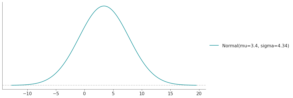

References

preliz.unidimensional.quartile(distribution=None, q1=-1, q2=0, q3=1, fixed_params=None, plot=None, plot_kwargs=None, ax=None)[source]#

Find the distribution with the specified quartiles.

Parameters:

distribution (PreliZ or PyMC distribution) – PreliZ distribution are updated inplace, while PyMC distributions are converted to PreliZ distributions. Distributions can be partially initialized, i.e. some parameters can be fixed while others are left free to be estimated. For PreliZ distributions, set the parameters you want to fix and don’t set the rest. As an alternative fixed_params can be used. For PyMC distributions, set the parameters to np.nan, and use fixed_params in case you want to fix any of them.
q1 (float) – First quartile, i.e 0.25 of the mass is below this point.
q2 (float) – Second quartile, i.e 0.50 of the mass is below this point. This is also know as the median.
q3 (float) – Third quartile, i.e 0.75 of the mass is below this point.
fixed_params (dict) – Dictionary with parameter names as keys and the values to fix them to as values. If using a PreliZ distribution, parameters can also be fixed by setting them when initializing the distribution. Defaults to None.
plot (bool) – Whether to plot the distribution, and lower and upper bounds. Defaults to None, which results in the value of rcParams[“plots.show_plot”] being used.
plot_kwargs (dict) – Dictionary passed to the method plot_pdf() of distribution.
ax (matplotlib axes)

Returns:

dict (dict with the parameters of the distribution)
axes (matplotlib axes (only if plot=True))

Notes

After calling this function the attribute opt of the distribution will be updated with the OptimizeResult object from the optimization step.

See also

maxent: Find the maximum entropy distribution with a given mass inside a user defined interval.

Examples

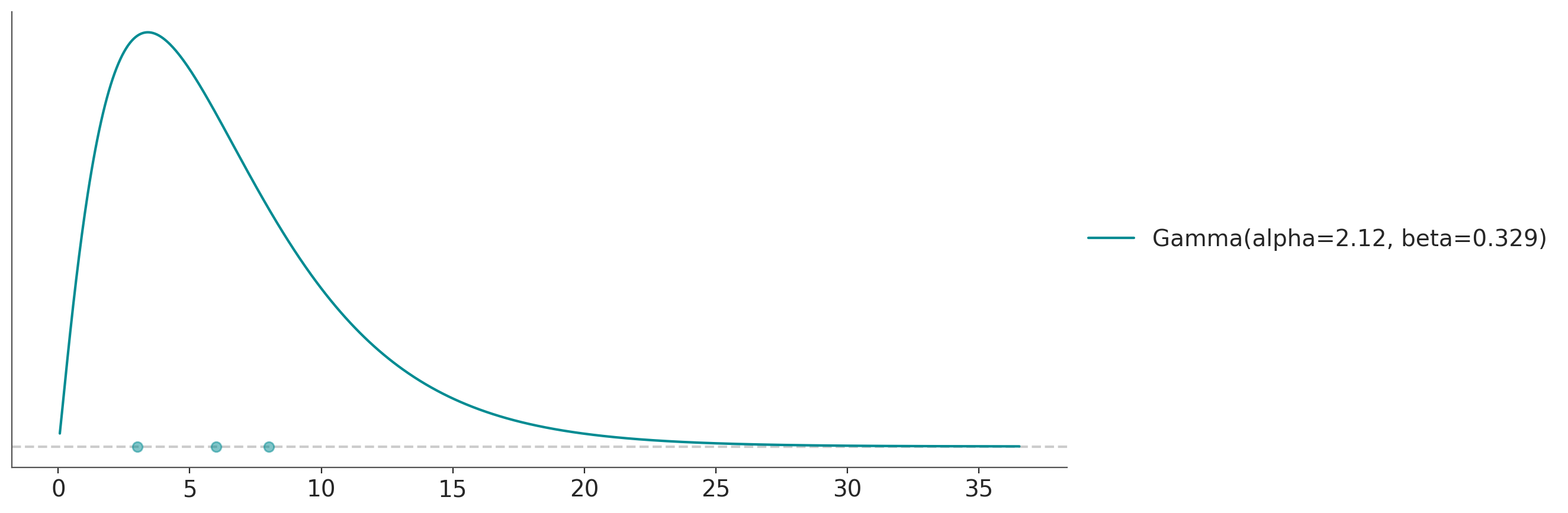
Calculate the Gamma distribution with quartiles 3, 6 and 8:

>>> import preliz as pz
>>> pz.style.use('preliz-doc')
>>> pz.quartile(pz.Gamma(), 3, 6, 8)

(Source code, png, hires.png, pdf)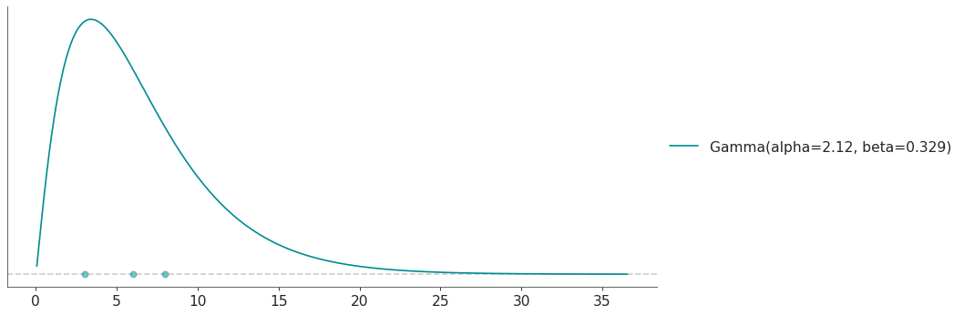

Calculate the HalfStudentT T distribution with quartiles 2, 9 and 12 and a value of nu=7:

>>> import preliz as pz
>>> pz.style.use('preliz-doc')
>>> pz.quartile(pz.HalfStudentT(nu=7), 2, 9, 12)

(Source code, png, hires.png, pdf)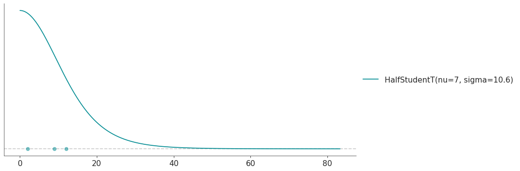

Unidimensional#

preliz.unidimensional#

`preliz.unidimensional`#